Counterfactual Analysis in a Medical Case

In this example we examine a case where we want to ask counterfactual questions, for events that have already taken place. We focus on a tele-medicine example related to eye-sight problems, where we know the causal structure of three observed variables and we want to ask counterfactual questions based of the type “What would have happened had I followed a different approach of what the tele-medicine app had proposed?”.

More specifically, we consider the following case. Alice who experiences intense eye-dryness decides to use a tele-medicine online platform, as she is not able to visit an eye doctor where she lives. She goes through the steps of reporting her medical history that reveals whether Alice has a rare allergy or not and the platform in the end recommends her two possible eye drops, with slightly different ingredients (‘option 1’ and ‘option 2’). Alice does a quick search online, and she finds that there are many positive reviews for option 1. Nevertheless, she decides to use option 2 as her mother has also used it in the past, and it had positive results. After a couple of days Alice’s vision becomes much better and her symptoms start to disappear. However, she is very curious what would have happened if she had used the very popular option 1 instead, or even did nothing.

The platform provides the possibility for the user to ask counterfactual questions as long as they report the outcome of the option they followed.

The data

We are having a database consisting of three observed variables: A continuous variable from 0 to 1 that indicates the quality of eyesight (‘Vision’), a binary variable that indicates whether a patient has a rare condition (i.e. allergy) or not (‘Condition’), and a categorical variable (‘Treatment’) that can take three values (0: ‘Do nothing’, 1: ‘option 1’ or 2: ‘option 2’). The data looks like this:

import pandas as pd

medical_data = pd.read_csv('patients_database.csv')
medical_data.head()

	Condition	Treatment	Vision
0	0	2	0.111728
1	0	0	0.191516
2	0	2	0.163924
3	0	1	0.886563
4	0	1	0.761090

medical_data.iloc[0:100].plot(figsize=(15, 10))

<Axes: >

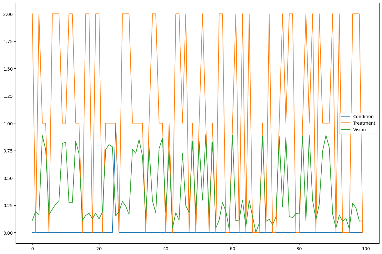
The dataset reflects the Vision of patients after they have taken one of the three Treatment options based on whether they have the rare Condition or not. Notice that the dataset has no information about the original vision of the patients (i.e. the noise of the Vision variable) before the treatment. As we will see below, this noise part of the vision is being recovered by the counterfactual algorithm as long as we have a post-nonlinear model (e.g. an ANM). The structural causal model used for the generation of the data is explained in detail in the Appendix. Each of these three observed nodes has an intrinsic noise, which is not observed.

Modeling of the graph

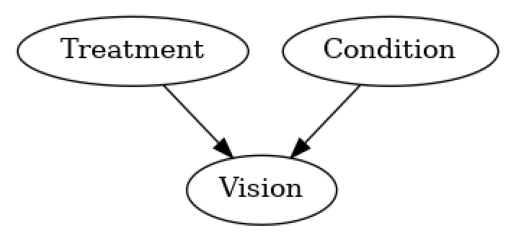
We know that the Treatment node and the Condition node are causing the Vision, but we don’t know the structural causal model. However, we can learn it from the observed data and, in particular, as long as post non-linear model assumption is not violated, we are able to reconstruct the noise for a particular observation. We assume that this graph is correctly representing the causal relationships, and we assume that there are no hidden confounders (causal sufficiency). Based on the given graph and data, we can then fit the causal model and start answering counterfactual questions.

import networkx as nx
import dowhy.gcm as gcm
from dowhy.utils import plot

causal_model = gcm.InvertibleStructuralCausalModel(nx.DiGraph([('Treatment', 'Vision'), ('Condition', 'Vision')]))
gcm.auto.assign_causal_mechanisms(causal_model, medical_data)

plot(causal_model.graph)

gcm.fit(causal_model, medical_data)

Fitting causal mechanism of node Condition: 100%|██████████| 3/3 [00:00<00:00, 17.59it/s]

Optionally, we can now also evaluate the fitted causal model:

print(gcm.evaluate_causal_model(causal_model, medical_data))

Evaluating causal mechanisms...: 100%|██████████| 3/3 [00:00<00:00, 4094.67it/s]
Test permutations of given graph: 100%|██████████| 6/6 [00:00<00:00, 89.59it/s]

Evaluated the performance of the causal mechanisms and the invertibility assumption of the causal mechanisms and the overall average KL divergence between generated and observed distribution and the graph structure. The results are as follows:

==== Evaluation of Causal Mechanisms ====
The used evaluation metrics are:
- KL divergence (only for root-nodes): Evaluates the divergence between the generated and the observed distribution.
- Mean Squared Error (MSE): Evaluates the average squared differences between the observed values and the conditional expectation of the causal mechanisms.
- Normalized MSE (NMSE): The MSE normalized by the standard deviation for better comparison.
- R2 coefficient: Indicates how much variance is explained by the conditional expectations of the mechanisms. Note, however, that this can be misleading for nonlinear relationships.
- F1 score (only for categorical non-root nodes): The harmonic mean of the precision and recall indicating the goodness of the underlying classifier model.
- (normalized) Continuous Ranked Probability Score (CRPS): The CRPS generalizes the Mean Absolute Percentage Error to probabilistic predictions. This gives insights into the accuracy and calibration of the causal mechanisms.
NOTE: Every metric focuses on different aspects and they might not consistently indicate a good or bad performance.
We will mostly utilize the CRPS for comparing and interpreting the performance of the mechanisms, since this captures the most important properties for the causal model.

--- Node Treatment
- The KL divergence between generated and observed distribution is 0.0.
The estimated KL divergence indicates an overall very good representation of the data distribution.

--- Node Condition
- The KL divergence between generated and observed distribution is 0.0.
The estimated KL divergence indicates an overall very good representation of the data distribution.

--- Node Vision
- The MSE is 0.0032632730427875596.
- The NMSE is 0.1825865878989047.
- The R2 coefficient is 0.9666554114523562.
- The normalized CRPS is 0.10644916945576403.
The estimated CRPS indicates a very good model performance.

==== Evaluation of Invertible Functional Causal Model Assumption ====

--- The model assumption for node Vision is not rejected with a p-value of 1.0 (after potential adjustment) and a significance level of 0.05.
This implies that the model assumption might be valid.

Note that these results are based on statistical independence tests, and the fact that the assumption was not rejected does not necessarily imply that it is correct. There is just no evidence against it.

==== Evaluation of Generated Distribution ====
The overall average KL divergence between the generated and observed distribution is 0.0
The estimated KL divergence indicates an overall very good representation of the data distribution.

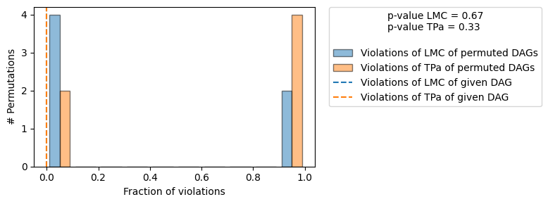
==== Evaluation of the Causal Graph Structure ====
+-------------------------------------------------------------------------------------------------------+
|                                         Falsificaton Summary                                          |
+-------------------------------------------------------------------------------------------------------+
| The given DAG is not informative because 2 / 6 of the permutations lie in the Markov                  |
| equivalence class of the given DAG (p-value: 0.33).                                                   |
| The given DAG violates 0/2 LMCs and is better than 33.3% of the permuted DAGs (p-value: 0.67).        |
| Based on the provided significance level (0.2) and because the DAG is not informative,                |
| we do not reject the DAG.                                                                             |
+-------------------------------------------------------------------------------------------------------+

==== NOTE ====
Always double check the made model assumptions with respect to the graph structure and choice of causal mechanisms.
All these evaluations give some insight into the goodness of the causal model, but should not be overinterpreted, since some causal relationships can be intrinsically hard to model. Furthermore, many algorithms are fairly robust against misspecifications or poor performances of causal mechanisms.

This confirms the accuracy of our causal model.

Now returning to our original problem, let’s load Alice’s data, who happens to have a rare allergy (Condition = 1).

specific_patient_data = pd.read_csv('newly_come_patients.csv')
specific_patient_data.head()

	Condition	Treatment	Vision
0	1	2	0.883874

Answering Alice’s counterfactual queries

In cases where we want to examine a hypothetical outcome if an event had not happened or if it had happened differently, we employ the so-called Counterfactual logic based on structural causal models. Given: - We know Alice’s treatment was option 2. - Alice has the rare allergy (Condition=1). - Alice vision is 0.78 (Vision=0.78) after treatment option 2. - We are able to recover the noise based on the learned structural causal model.

We can now examine the counterfactual outcome for her Vision if the Treatment node had been different. In the following, we look at the counterfactual value for Vision of Alice if she had taken no treatment (Treatment=0) and if she had taken the other eye drops (Treatment=1).

counterfactual_data1 = gcm.counterfactual_samples(causal_model,
                                                  {'Treatment': lambda x: 1},
                                                  observed_data = specific_patient_data)

counterfactual_data2 = gcm.counterfactual_samples(causal_model,
                                                  {'Treatment': lambda x: 0},
                                                  observed_data = specific_patient_data)


import matplotlib.pyplot as plt

df_plot2 = pd.DataFrame()
df_plot2['Vision after option 2'] = specific_patient_data['Vision']
df_plot2['Counterfactual vision (option 1)'] = counterfactual_data1['Vision']
df_plot2['Counterfactual vision (No treatment)'] = counterfactual_data2['Vision']

df_plot2.plot.bar(title="Counterfactual outputs")
plt.xlabel('Alice')
plt.ylabel('Eyesight quality')
plt.legend()

<matplotlib.legend.Legend at 0x7fb751d62bb0>

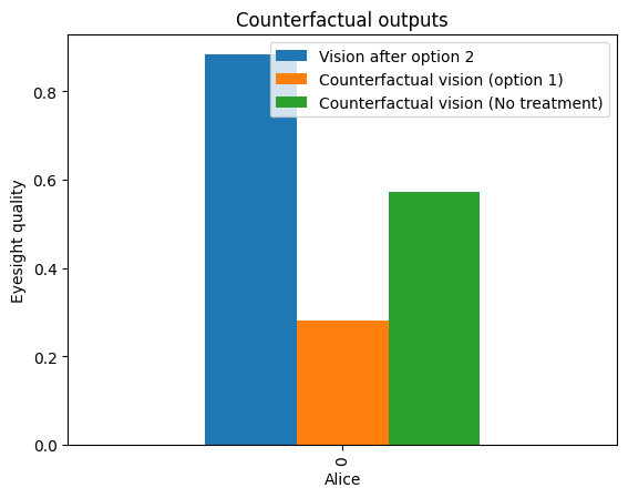
What we see here is that if Alice had taken option 1 instead, her Vision would have become worse compared to option 2. Therefore, she realised that the rare condition (Condition=1) that she had reported in her medical history could be the one that would have caused an allergic reaction to the popular option 1. Alice was also able to see that if she had not taken any of the recommended options, she would have resulted with worse eyesight (the variable Vision resulted in a smaller relative value) than with option 2 that she took.

Appendix: What the tele-app uses internally. Data generation of the patients’ log

Here we describe the SCM \(f_{p1, p2}\) for the additive noise model: \(Vision = N_V + f_{p1, p2}(Treatment, Condition)\). We sample the intrinsic additive noise for the three observed variables \(N_T, N_C\) and \(N_V\). The target variable Vision is then the additive noise \(N_V\) plus the function of its inputs nodes as described below.

\(Treatment = N_T\) ~ 0 , 1 or 2 with probabilities 33% respectively : 33% of the users do nothing, 33% take option 1 and 33% take option 2. This is independent of whether the patient has the rare condition.

\(Condition = N_C\) ~ Bernoulli(0.01) : whether the patient has the rare condition

$Vision = N_V + f_{p1, p2}(Treatment, Condition) = N_V - P_1(1 - Condition)(1-Treatment)(2-Treatment) + 2P_2(1-Condition)Treatment(2-Treatment) + P_2(1-Condition)(3-Treatment)(1-Treatment)Treatment - 2P_2 Condition Treatment(2-Treatment) - P_2 Condition(3-Treatment)(1-Treatment)Treatment $ patient’s vision, where:

\(P_1\) is a constant by which the original vision will be decreased in case the patient does not have the rare condition and he is not administrated any medicine.

\(P_2\) is a constant by which the original vision will be increased or decreased accordingly depending on whether the patient has the condition and the type of drops they will be administrated. More specifically:

If Condition = 0 and Treatment = 1 then Vision = N_V + P_2

elIf Condition = 0 and Treatment = 2 then Vision = N_V - P_2

elIf Condition = 1 and Treatment = 1 then Vision = N_V - P_2

elIf Condition = 1 and Treatment = 2 then Vision = N_V + P_2

elIf Condition = 0 and Treatment = 0 then Vision = N_V - P_1

elif Condition = 1 and Treatment = 0 then Vision = N_V - P3

NOTE It is important that the assigned functional causal models are invertible with respect to the noise (e.g. an additive noise model) for counterfactual statements. Alternatively, the user could also specify the ground truth models and ground truth noise.

For such rare events like having the condition (Condition=1, which has a low probability of 1%) it is necessary to have a lot of samples to train the model in order to accurately reflect these rare events. This is why here we used 10000 samples to generate the patients’ database.

from scipy.stats import bernoulli, norm, uniform
import numpy as np
from random import randint

n_unobserved = 10000
unobserved_data = {
   'N_T': np.array([randint(0, 2) for p in range(n_unobserved)]),
   'N_vision': np.random.uniform(0.4, 0.6, size=(n_unobserved,)),
   'N_C': bernoulli.rvs(0.01, size=n_unobserved)
}
P_1 = 0.2
P_2 = 0.15

def create_observed_medical_data(unobserved_data):
    observed_medical_data = {}
    observed_medical_data['Condition'] = unobserved_data['N_C']
    observed_medical_data['Treatment'] = unobserved_data['N_T']
    observed_medical_data['Vision'] = unobserved_data['N_vision'] + (-P_1)*(1 - observed_medical_data['Condition'])*(1 - observed_medical_data['Treatment'])*(2 - observed_medical_data['Treatment']) + (2*P_2)*(1 - observed_medical_data['Condition'])*(observed_medical_data['Treatment'])*(2 - observed_medical_data['Treatment']) + (P_2)*(1 - observed_medical_data['Condition'])*(observed_medical_data['Treatment'])*(1 - observed_medical_data['Treatment'])*(3 - observed_medical_data['Treatment']) + 0*(observed_medical_data['Condition'])*(1 - observed_medical_data['Treatment'])*(2 - observed_medical_data['Treatment']) + (-2*P_2)*(unobserved_data['N_C'])*(observed_medical_data['Treatment'])*(2 - observed_medical_data['Treatment']) + (-P_2)*(observed_medical_data['Condition'])*(observed_medical_data['Treatment'])*(1 - observed_medical_data['Treatment'])*(3 - observed_medical_data['Treatment'])
    return pd.DataFrame(observed_medical_data)

medical_data = create_observed_medical_data(unobserved_data)

Generate Alice’s data: A random noise for her initial vision, Condition=1 (as she has the rare allergy) and her initial decision to take Treatment=2 (eye drops option 2).

num_samples = 1
original_vision = np.random.uniform(0.4, 0.6, size=num_samples)
def generate_specific_patient_data(num_samples):
    return create_observed_medical_data({
    'N_T': np.full((num_samples,), 2),
    'N_C': bernoulli.rvs(1, size=num_samples),
    'N_vision': original_vision,
})

specific_patient_data = generate_specific_patient_data(num_samples)