Demo for the DoWhy causal API

We show a simple example of adding a causal extension to any dataframe.

import dowhy
dowhy.enable_notebook_rendering()

import dowhy.datasets
import dowhy.api
from dowhy.graph import build_graph_from_str

import numpy as np
import pandas as pd

from statsmodels.api import OLS

data = dowhy.datasets.linear_dataset(beta=5,
        num_common_causes=1,
        num_instruments = 0,
        num_samples=1000,
        treatment_is_binary=True)
df = data['df']
df['y'] = df['y'] + np.random.normal(size=len(df)) # Adding noise to data. Without noise, the variance in Y|X, Z is zero, and mcmc fails.
nx_graph = build_graph_from_str(data["dot_graph"])

treatment= data["treatment_name"][0]
outcome = data["outcome_name"][0]
common_cause = data["common_causes_names"][0]
df

	W0	v0	y
0	-1.732188	False	-5.246686
1	-1.434387	False	-2.697610
2	0.079443	False	-0.528697
3	0.354686	True	4.635497
4	0.565750	False	2.045890
...	...	...	...
995	-1.317844	True	2.172462
996	-0.496093	True	3.691537
997	-0.655248	False	-2.422656
998	-0.842732	False	-2.895357
999	0.396762	True	6.072133

1000 rows × 3 columns

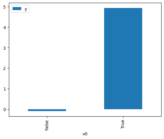
# data['df'] is just a regular pandas.DataFrame
df.causal.do(x=treatment,
             variable_types={treatment: 'b', outcome: 'c', common_cause: 'c'},
             outcome=outcome,
             common_causes=[common_cause],
            ).groupby(treatment).mean().plot(y=outcome, kind='bar')

<Axes: xlabel='v0'>

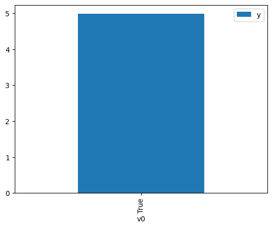
df.causal.do(x={treatment: 1},
              variable_types={treatment:'b', outcome: 'c', common_cause: 'c'},
              outcome=outcome,
              method='weighting',
              common_causes=[common_cause]
              ).groupby(treatment).mean().plot(y=outcome, kind='bar')

<Axes: xlabel='v0'>

cdf_1 = df.causal.do(x={treatment: 1},
              variable_types={treatment: 'b', outcome: 'c', common_cause: 'c'},
              outcome=outcome,
              graph=nx_graph
              )

cdf_0 = df.causal.do(x={treatment: 0},
              variable_types={treatment: 'b', outcome: 'c', common_cause: 'c'},
              outcome=outcome,
              graph=nx_graph
              )

cdf_0

	W0	v0	y	propensity_score	weight
0	0.167766	False	0.192205	0.521148	1.918839
1	-2.329915	False	-4.704267	0.573713	1.743031
2	-0.150972	False	1.779593	0.527907	1.894272
3	1.211190	False	3.125638	0.498981	2.004085
4	-2.334465	False	-4.964374	0.573808	1.742744
...	...	...	...	...	...
995	-1.206060	False	-0.465808	0.550195	1.817538
996	-0.114061	False	0.446756	0.527125	1.897083
997	-1.915985	False	-4.099968	0.565084	1.769648
998	-0.540436	False	-3.416089	0.536152	1.865142
999	0.899184	False	3.290114	0.505613	1.977797

1000 rows × 5 columns

cdf_1

	W0	v0	y	propensity_score	weight
0	1.332591	True	8.444178	0.503600	1.985704
1	-0.835955	True	2.419318	0.457605	2.185291
2	0.280999	True	5.656745	0.481255	2.077902
3	-0.979426	True	2.081329	0.454579	2.199839
4	0.542872	True	6.730109	0.486816	2.054166
...	...	...	...	...	...
995	1.072684	True	6.664267	0.498075	2.007730
996	1.758648	True	7.552956	0.512654	1.950635
997	0.133982	True	7.071244	0.478135	2.091461
998	-0.679531	True	2.922756	0.460908	2.169631
999	-0.680970	True	4.373189	0.460878	2.169774

1000 rows × 5 columns

Comparing the estimate to Linear Regression

First, estimating the effect using the causal data frame, and the 95% confidence interval.

(cdf_1['y'] - cdf_0['y']).mean()

$\displaystyle 5.14894251033807$

1.96*(cdf_1['y'] - cdf_0['y']).std() / np.sqrt(len(df))

$\displaystyle 0.217294994027793$

Comparing to the estimate from OLS.

model = OLS(np.asarray(df[outcome]), np.asarray(df[[common_cause, treatment]], dtype=np.float64))
result = model.fit()
result.summary()

OLS Regression Results

Dep. Variable:	y	R-squared (uncentered):	0.938
Model:	OLS	Adj. R-squared (uncentered):	0.938
Method:	Least Squares	F-statistic:	7563.
Date:	Thu, 11 Jun 2026	Prob (F-statistic):	0.00
Time:	19:09:04	Log-Likelihood:	-1415.2
No. Observations:	1000	AIC:	2834.
Df Residuals:	998	BIC:	2844.
Df Model:	2
Covariance Type:	nonrobust

	coef	std err	t	P>|t|	[0.025	0.975]
x1	2.1256	0.031	68.253	0.000	2.064	2.187
x2	4.9357	0.046	107.210	0.000	4.845	5.026

Omnibus:	1.422	Durbin-Watson:	1.985
Prob(Omnibus):	0.491	Jarque-Bera (JB):	1.285
Skew:	0.062	Prob(JB):	0.526
Kurtosis:	3.125	Cond. No.	1.49

Notes:
[1] R² is computed without centering (uncentered) since the model does not contain a constant.
[2] Standard Errors assume that the covariance matrix of the errors is correctly specified.