Simple example on using Instrumental Variables method for estimation#
[1]:
%load_ext autoreload
%autoreload 2
[2]:
import dowhy
dowhy.enable_notebook_rendering()

import numpy as np
import pandas as pd
import patsy as ps

from statsmodels.sandbox.regression.gmm import IV2SLS
import os, sys
from dowhy import CausalModel
Loading the dataset#
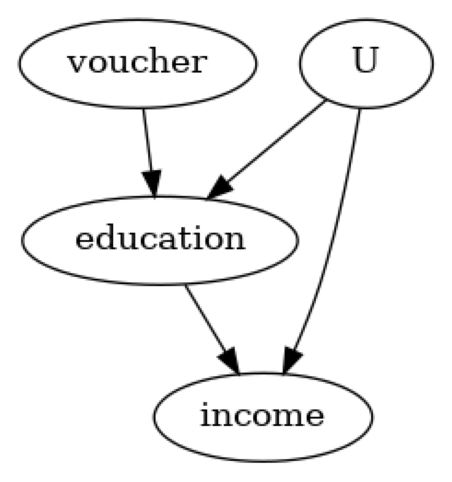
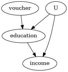
We create a fictitious dataset with the goal of estimating the impact of education on future earnings of an individual. The ability of the individual is a confounder and being given an education_voucher is the instrument.
[3]:
n_points = 1000
education_abilty = 1
education_voucher = 2
income_abilty = 2
income_education = 4


# confounder
ability = np.random.normal(0, 3, size=n_points)

# instrument
voucher = np.random.normal(2, 1, size=n_points)

# treatment
education = np.random.normal(5, 1, size=n_points) + education_abilty * ability +\
            education_voucher * voucher

# outcome
income = np.random.normal(10, 3, size=n_points) +\
         income_abilty * ability + income_education * education

# build dataset (exclude confounder `ability` which we assume to be unobserved)
data = np.stack([education, income, voucher]).T
df = pd.DataFrame(data, columns = ['education', 'income', 'voucher'])
Using DoWhy to estimate the causal effect of education on future income#
We follow the four steps:
model the problem using causal graph,
identify if the causal effect can be estimated from the observed variables,
estimate the effect, and
check the robustness of the estimate.
[4]:
#Step 1: Model
model=CausalModel(
        data = df,
        treatment='education',
        outcome='income',
        common_causes=['U'],
        instruments=['voucher']
        )
model.view_model()
from IPython.display import Image, display
display(Image(filename="causal_model.png"))
/home/runner/work/dowhy/dowhy/dowhy/causal_model.py:577: UserWarning: 1 variables are assumed unobserved because they are not in the dataset. Configure the logging level to `logging.WARNING` or higher for additional details.
  warnings.warn(
[5]:
# Step 2: Identify
identified_estimand = model.identify_effect(proceed_when_unidentifiable=True)
print(identified_estimand)
Estimand type: EstimandType.NONPARAMETRIC_ATE

### Estimand : 1
Estimand name: backdoor
No such variable(s) found!

### Estimand : 2
Estimand name: iv
Estimand expression:
 ⎡                                            -1⎤
 ⎢    d              ⎛    d                  ⎞  ⎥
E⎢──────────(income)⋅⎜──────────([education])⎟  ⎥
 ⎣d[voucher]         ⎝d[voucher]             ⎠  ⎦
Estimand assumption 1, As-if-random: If U→→income then ¬(U →→{voucher})
Estimand assumption 2, Exclusion: If we remove {voucher}→{education}, then ¬({voucher}→income)

### Estimand : 3
Estimand name: frontdoor
No such variable(s) found!
[6]:
# Step 3: Estimate
#Choose the second estimand: using IV
estimate = model.estimate_effect(identified_estimand,
        method_name="iv.instrumental_variable", test_significance=True)

print(estimate)
*** Causal Estimate ***

## Identified estimand
Estimand type: EstimandType.NONPARAMETRIC_ATE

### Estimand : 1
Estimand name: iv
Estimand expression:
 ⎡                                            -1⎤
 ⎢    d              ⎛    d                  ⎞  ⎥
E⎢──────────(income)⋅⎜──────────([education])⎟  ⎥
 ⎣d[voucher]         ⎝d[voucher]             ⎠  ⎦
Estimand assumption 1, As-if-random: If U→→income then ¬(U →→{voucher})
Estimand assumption 2, Exclusion: If we remove {voucher}→{education}, then ¬({voucher}→income)

## Realized estimand
Realized estimand: Wald Estimator
Realized estimand type: EstimandType.NONPARAMETRIC_ATE
Estimand expression:
  ⎡   d            ⎤
 E⎢────────(income)⎥
  ⎣dvoucher        ⎦
──────────────────────
 ⎡   d               ⎤
E⎢────────(education)⎥
 ⎣dvoucher           ⎦
Estimand assumption 1, As-if-random: If U→→income then ¬(U →→{voucher})
Estimand assumption 2, Exclusion: If we remove {voucher}→{education}, then ¬({voucher}→income)
Estimand assumption 3, treatment_effect_homogeneity: Each unit's treatment ['education'] is affected in the same way by common causes of ['education'] and ['income']
Estimand assumption 4, outcome_effect_homogeneity: Each unit's outcome ['income'] is affected in the same way by common causes of ['education'] and ['income']

Target units: ate

## Estimate
Mean value: 3.9524136618777415
p-value: [0, 0.001]
We have an estimate, indicating that increasing education by one unit increases income by 4 points.
Next we check the robustness of the estimate using a Placebo refutation test. In this test, the treatment is replaced by an independent random variable (while preserving the correlation with the instrument), so that the true causal effect should be zero. We check if our estimator also provides the correct answer of zero.
[7]:
# Step 4: Refute
ref = model.refute_estimate(identified_estimand, estimate, method_name="placebo_treatment_refuter", placebo_type="permute") # only permute placebo_type works with IV estimate
print(ref)
Refute: Use a Placebo Treatment
Estimated effect:3.9524136618777415
New effect:-0.06986683469294354
p value:0.66
The refutation gives confidence that the estimate is not capturing any noise in the data.
Since this is simulated data, we also know the true causal effect is 4 (see the income_education parameter of the data-generating process above)
Finally, we show the same estimation by another method to verify the result from DoWhy.
[8]:
income_vec, endog = ps.dmatrices("income ~ education", data=df)
exog = ps.dmatrix("voucher", data=df)

m = IV2SLS(income_vec, endog, exog).fit()
m.summary()
[8]:
| Dep. Variable: | income | R-squared: | 0.882 |
|---|---|---|---|
| Model: | IV2SLS | Adj. R-squared: | 0.882 |
| Method: | Two Stage | F-statistic: | 1265. |
| Least Squares | Prob (F-statistic): | 1.41e-179 | |
| Date: | Sat, 13 Jun 2026 | ||
| Time: | 20:11:56 | ||
| No. Observations: | 1000 | ||
| Df Residuals: | 998 | ||
| Df Model: | 1 |
| coef | std err | t | P>|t| | [0.025 | 0.975] | |
|---|---|---|---|---|---|---|
| Intercept | 10.3724 | 1.017 | 10.199 | 0.000 | 8.377 | 12.368 |
| education | 3.9524 | 0.111 | 35.560 | 0.000 | 3.734 | 4.171 |
| Omnibus: | 0.616 | Durbin-Watson: | 2.088 |
|---|---|---|---|
| Prob(Omnibus): | 0.735 | Jarque-Bera (JB): | 0.703 |
| Skew: | 0.038 | Prob(JB): | 0.704 |
| Kurtosis: | 2.894 | Cond. No. | 25.6 |