Estimating effect of multiple treatments#
[1]:
import dowhy
dowhy.enable_notebook_rendering()

from dowhy import CausalModel
import dowhy.datasets

import warnings
warnings.filterwarnings('ignore')
[2]:
data = dowhy.datasets.linear_dataset(10, num_common_causes=4, num_samples=10000,
                                     num_instruments=0, num_effect_modifiers=2,
                                     num_treatments=2,
                                     treatment_is_binary=False,
                                     num_discrete_common_causes=2,
                                     num_discrete_effect_modifiers=0,
                                     one_hot_encode=False)
df=data['df']
df.head()
[2]:
| X0 | X1 | W0 | W1 | W2 | W3 | v0 | v1 | y | |
|---|---|---|---|---|---|---|---|---|---|
| 0 | 1.936960 | 1.286461 | -0.437094 | 0.546103 | 0 | 1 | 3.303197 | 6.708500 | 321.455093 |
| 1 | 1.234611 | 1.281467 | -0.573464 | 1.417379 | 2 | 3 | 16.751182 | 19.842095 | 2763.462466 |
| 2 | 1.464677 | 2.631633 | -1.132205 | -0.432581 | 3 | 3 | 12.162636 | 9.412274 | 1431.418856 |
| 3 | -0.320451 | -0.231835 | 0.748453 | -0.143496 | 3 | 3 | 19.441933 | 15.639146 | -150.664756 |
| 4 | 1.056271 | 0.767362 | 0.713936 | -0.089138 | 3 | 1 | 15.796937 | 8.035628 | 952.033549 |
[3]:
model = CausalModel(data=data["df"],
                    treatment=data["treatment_name"], outcome=data["outcome_name"],
                    graph=data["gml_graph"])
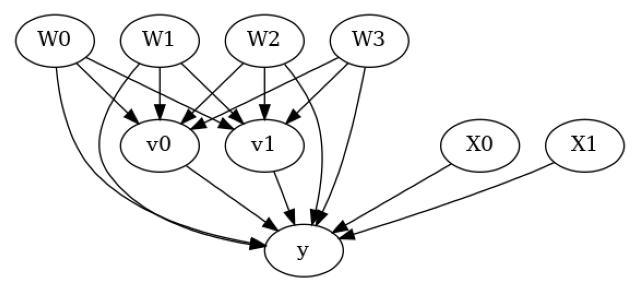
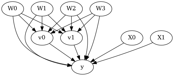
[4]:
model.view_model()
from IPython.display import Image, display
display(Image(filename="causal_model.png"))
[5]:
identified_estimand= model.identify_effect(proceed_when_unidentifiable=True)
print(identified_estimand)
Estimand type: EstimandType.NONPARAMETRIC_ATE

### Estimand : 1
Estimand name: backdoor
Estimand expression:
    d
─────────(E[y|W3,W1,W2,W0])
d[v₀  v₁]
Estimand assumption 1, Unconfoundedness: If U→{v0,v1} and U→y then P(y|v0,v1,W3,W1,W2,W0,U) = P(y|v0,v1,W3,W1,W2,W0)

### Estimand : 2
Estimand name: iv
No such variable(s) found!

### Estimand : 3
Estimand name: frontdoor
No such variable(s) found!
Linear model#
Let us first see an example for a linear model. The control_value and treatment_value can be provided as a tuple/list when the treatment is multi-dimensional.
The interpretation is change in y when v0 and v1 are changed from (0,0) to (1,1).
[6]:
linear_estimate = model.estimate_effect(identified_estimand,
                                        method_name="backdoor.linear_regression",
                                        control_value=(0,0),
                                        treatment_value=(1,1),
                                        method_params={'need_conditional_estimates': False})
print(linear_estimate)
*** Causal Estimate ***

## Identified estimand
Estimand type: EstimandType.NONPARAMETRIC_ATE

### Estimand : 1
Estimand name: backdoor
Estimand expression:
    d
─────────(E[y|W3,W1,W2,W0])
d[v₀  v₁]
Estimand assumption 1, Unconfoundedness: If U→{v0,v1} and U→y then P(y|v0,v1,W3,W1,W2,W0,U) = P(y|v0,v1,W3,W1,W2,W0)

## Realized estimand
b: y~v0+v1+W3+W1+W2+W0+v0*X0+v0*X1+v1*X0+v1*X1
Target units: ate

## Estimate
Mean value: 87.21424346164285
You can estimate conditional effects, based on effect modifiers.
[7]:
linear_estimate = model.estimate_effect(identified_estimand,
                                        method_name="backdoor.linear_regression",
                                        control_value=(0,0),
                                        treatment_value=(1,1))
print(linear_estimate)
*** Causal Estimate ***

## Identified estimand
Estimand type: EstimandType.NONPARAMETRIC_ATE

### Estimand : 1
Estimand name: backdoor
Estimand expression:
    d
─────────(E[y|W3,W1,W2,W0])
d[v₀  v₁]
Estimand assumption 1, Unconfoundedness: If U→{v0,v1} and U→y then P(y|v0,v1,W3,W1,W2,W0,U) = P(y|v0,v1,W3,W1,W2,W0)

## Realized estimand
b: y~v0+v1+W3+W1+W2+W0+v0*X0+v0*X1+v1*X0+v1*X1
Target units:

## Estimate
Mean value: 87.21424346164285
### Conditional Estimates
__categorical__X0  __categorical__X1
(-2.717, 0.0741]   (-3.2359999999999998, -0.282]    -12.475222
                   (-0.282, 0.307]                    6.545126
                   (0.307, 0.822]                    18.924325
                   (0.822, 1.404]                    29.659636
                   (1.404, 4.283]                    50.856796
(0.0741, 0.646]    (-3.2359999999999998, -0.282]     28.470841
                   (-0.282, 0.307]                   49.228702
                   (0.307, 0.822]                    60.296887
                   (0.822, 1.404]                    72.744082
                   (1.404, 4.283]                    91.796687
(0.646, 1.158]     (-3.2359999999999998, -0.282]     55.511858
                   (-0.282, 0.307]                   74.525618
                   (0.307, 0.822]                    86.336480
                   (0.822, 1.404]                    98.421848
                   (1.404, 4.283]                   118.012793
(1.158, 1.755]     (-3.2359999999999998, -0.282]     81.975942
                   (-0.282, 0.307]                  100.465067
                   (0.307, 0.822]                   113.495952
                   (0.822, 1.404]                   124.152992
                   (1.404, 4.283]                   144.519310
(1.755, 4.452]     (-3.2359999999999998, -0.282]    126.722175
                   (-0.282, 0.307]                  146.043394
                   (0.307, 0.822]                   159.572426
                   (0.822, 1.404]                   168.369418
                   (1.404, 4.283]                   186.170311
dtype: float64
More methods#
You can also use methods from EconML or CausalML libraries that support multiple treatments. You can look at examples from the conditional effect notebook: https://py-why.github.io/dowhy/example_notebooks/dowhy-conditional-treatment-effects.html
Propensity-based methods do not support multiple treatments currently.