Confounding Example: Finding causal effects from observed data

Suppose you are given some data with treatment and outcome. Can you determine whether the treatment causes the outcome, or the correlation is purely due to another common cause?

import numpy as np
import pandas as pd
import matplotlib.pyplot as plt
import math
import dowhy
from dowhy import CausalModel
import dowhy.datasets, dowhy.plotter

# Config dict to set the logging level
import logging.config
DEFAULT_LOGGING = {
    'version': 1,
    'disable_existing_loggers': False,
    'loggers': {
        '': {
            'level': 'INFO',
        },
    }
}

logging.config.dictConfig(DEFAULT_LOGGING)

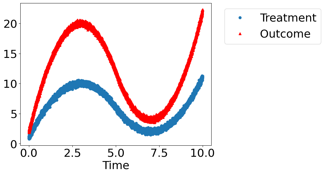
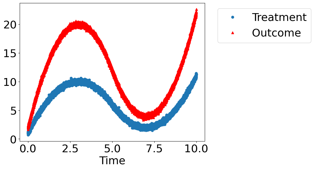
Let’s create a mystery dataset for which we need to determine whether there is a causal effect.

Creating the dataset. It is generated from either one of two models: * Model 1: Treatment does cause outcome. * Model 2: Treatment does not cause outcome. All observed correlation is due to a common cause.

rvar = 1 if np.random.uniform() >0.5 else 0
data_dict = dowhy.datasets.xy_dataset(10000, effect=rvar,
                                      num_common_causes=1,
                                      sd_error=0.2)
df = data_dict['df']
print(df[["Treatment", "Outcome", "w0"]].head())

   Treatment    Outcome        w0
0  10.387253  20.277407  3.965843
1   1.727999   4.197184 -3.995572
2   6.492521  13.045906  0.509105
3   2.002103   4.126254 -3.934166
4   6.728680  12.993550  0.480317

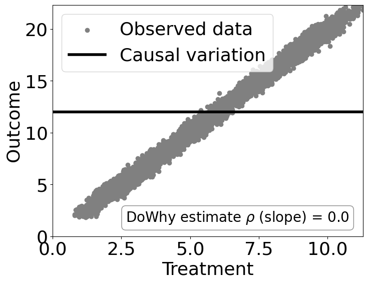
dowhy.plotter.plot_treatment_outcome(df[data_dict["treatment_name"]], df[data_dict["outcome_name"]],
                             df[data_dict["time_val"]])

Using DoWhy to resolve the mystery: Does Treatment cause Outcome?

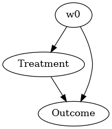
STEP 1: Model the problem as a causal graph

Initializing the causal model.

model= CausalModel(
        data=df,
        treatment=data_dict["treatment_name"],
        outcome=data_dict["outcome_name"],
        common_causes=data_dict["common_causes_names"],
        instruments=data_dict["instrument_names"])
model.view_model(layout="dot")

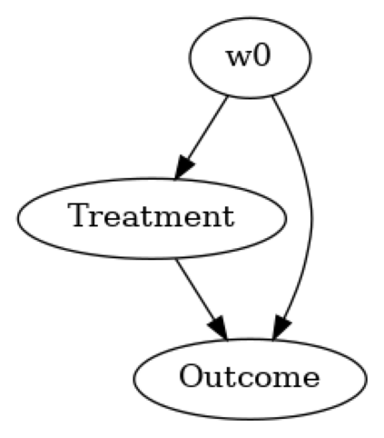
Showing the causal model stored in the local file “causal_model.png”

from IPython.display import Image, display
display(Image(filename="causal_model.png"))

STEP 2: Identify causal effect using properties of the formal causal graph

Identify the causal effect using properties of the causal graph.

identified_estimand = model.identify_effect(proceed_when_unidentifiable=True)
print(identified_estimand)

Estimand type: EstimandType.NONPARAMETRIC_ATE

### Estimand : 1
Estimand name: backdoor
Estimand expression:
     d
────────────(E[Outcome|w0])
d[Treatment]
Estimand assumption 1, Unconfoundedness: If U→{Treatment} and U→Outcome then P(Outcome|Treatment,w0,U) = P(Outcome|Treatment,w0)

### Estimand : 2
Estimand name: iv
No such variable(s) found!

### Estimand : 3
Estimand name: frontdoor
No such variable(s) found!

STEP 3: Estimate the causal effect

Once we have identified the estimand, we can use any statistical method to estimate the causal effect.

Let’s use Linear Regression for simplicity.

estimate = model.estimate_effect(identified_estimand,
        method_name="backdoor.linear_regression")
print("Causal Estimate is " + str(estimate.value))

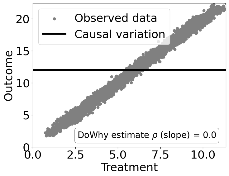
# Plot Slope of line between treamtent and outcome =causal effect
dowhy.plotter.plot_causal_effect(estimate, df[data_dict["treatment_name"]], df[data_dict["outcome_name"]])

Causal Estimate is 0.9920735448221185

Checking if the estimate is correct

print("DoWhy estimate is " + str(estimate.value))
print ("Actual true causal effect was {0}".format(rvar))

DoWhy estimate is 0.9920735448221185
Actual true causal effect was 1

Step 4: Refuting the estimate

We can also refute the estimate to check its robustness to assumptions (aka sensitivity analysis, but on steroids).

Adding a random common cause variable

res_random=model.refute_estimate(identified_estimand, estimate, method_name="random_common_cause")
print(res_random)

Refute: Add a random common cause
Estimated effect:0.9920735448221185
New effect:0.9920717339951729
p value:1.0

Replacing treatment with a random (placebo) variable

res_placebo=model.refute_estimate(identified_estimand, estimate,
        method_name="placebo_treatment_refuter", placebo_type="permute")
print(res_placebo)

Refute: Use a Placebo Treatment
Estimated effect:0.9920735448221185
New effect:0.00012804244976383217
p value:0.8600000000000001

Removing a random subset of the data

res_subset=model.refute_estimate(identified_estimand, estimate,
        method_name="data_subset_refuter", subset_fraction=0.9)
print(res_subset)

Refute: Use a subset of data
Estimated effect:0.9920735448221185
New effect:0.9926942324151313
p value:0.8799999999999999

As you can see, our causal estimator is robust to simple refutations.