Estimating effect of multiple treatments#
[1]:
from dowhy import CausalModel
import dowhy.datasets

import warnings
warnings.filterwarnings('ignore')
[2]:
data = dowhy.datasets.linear_dataset(10, num_common_causes=4, num_samples=10000,
                                     num_instruments=0, num_effect_modifiers=2,
                                     num_treatments=2,
                                     treatment_is_binary=False,
                                     num_discrete_common_causes=2,
                                     num_discrete_effect_modifiers=0,
                                     one_hot_encode=False)
df=data['df']
df.head()
[2]:
| X0 | X1 | W0 | W1 | W2 | W3 | v0 | v1 | y | |
|---|---|---|---|---|---|---|---|---|---|
| 0 | 0.695608 | 0.312661 | -0.021857 | -0.326661 | 3 | 1 | 3.922958 | 14.364549 | 349.237904 |
| 1 | 1.615299 | -1.272674 | -0.422047 | -2.091060 | 3 | 2 | -0.158817 | 10.393182 | 112.093624 |
| 2 | -1.701713 | 1.035348 | -0.172448 | -4.223078 | 3 | 1 | -5.915384 | -0.744664 | -78.030150 |
| 3 | -2.266305 | -0.856940 | 0.612950 | -1.612232 | 1 | 2 | 1.263043 | 1.886007 | 18.936871 |
| 4 | -1.404892 | -0.710122 | 2.164879 | -0.392689 | 1 | 0 | 3.781417 | 4.081440 | 0.287956 |
[3]:
model = CausalModel(data=data["df"],
                    treatment=data["treatment_name"], outcome=data["outcome_name"],
                    graph=data["gml_graph"])
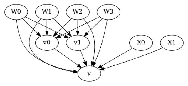
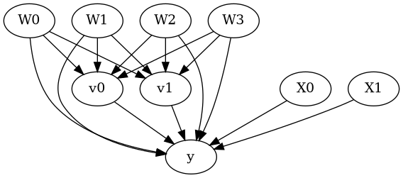
[4]:
model.view_model()
from IPython.display import Image, display
display(Image(filename="causal_model.png"))
[5]:
identified_estimand= model.identify_effect(proceed_when_unidentifiable=True)
print(identified_estimand)
Estimand type: EstimandType.NONPARAMETRIC_ATE

### Estimand : 1
Estimand name: backdoor
Estimand expression:
    d
─────────(E[y|W3,W0,W2,W1])
d[v₀  v₁]
Estimand assumption 1, Unconfoundedness: If U→{v0,v1} and U→y then P(y|v0,v1,W3,W0,W2,W1,U) = P(y|v0,v1,W3,W0,W2,W1)

### Estimand : 2
Estimand name: iv
No such variable(s) found!

### Estimand : 3
Estimand name: frontdoor
No such variable(s) found!
Linear model#
Let us first see an example for a linear model. The control_value and treatment_value can be provided as a tuple/list when the treatment is multi-dimensional.
The interpretation is change in y when v0 and v1 are changed from (0,0) to (1,1).
[6]:
linear_estimate = model.estimate_effect(identified_estimand,
                                        method_name="backdoor.linear_regression",
                                        control_value=(0,0),
                                        treatment_value=(1,1),
                                        method_params={'need_conditional_estimates': False})
print(linear_estimate)
*** Causal Estimate ***

## Identified estimand
Estimand type: EstimandType.NONPARAMETRIC_ATE

### Estimand : 1
Estimand name: backdoor
Estimand expression:
    d
─────────(E[y|W3,W0,W2,W1])
d[v₀  v₁]
Estimand assumption 1, Unconfoundedness: If U→{v0,v1} and U→y then P(y|v0,v1,W3,W0,W2,W1,U) = P(y|v0,v1,W3,W0,W2,W1)

## Realized estimand
b: y~v0+v1+W3+W0+W2+W1+v0*X0+v0*X1+v1*X0+v1*X1
Target units: ate

## Estimate
Mean value: 6.875864797841594
You can estimate conditional effects, based on effect modifiers.
[7]:
linear_estimate = model.estimate_effect(identified_estimand,
                                        method_name="backdoor.linear_regression",
                                        control_value=(0,0),
                                        treatment_value=(1,1))
print(linear_estimate)
*** Causal Estimate ***

## Identified estimand
Estimand type: EstimandType.NONPARAMETRIC_ATE

### Estimand : 1
Estimand name: backdoor
Estimand expression:
    d
─────────(E[y|W3,W0,W2,W1])
d[v₀  v₁]
Estimand assumption 1, Unconfoundedness: If U→{v0,v1} and U→y then P(y|v0,v1,W3,W0,W2,W1,U) = P(y|v0,v1,W3,W0,W2,W1)

## Realized estimand
b: y~v0+v1+W3+W0+W2+W1+v0*X0+v0*X1+v1*X0+v1*X1
Target units:

## Estimate
Mean value: 6.875864797841594
### Conditional Estimates
__categorical__X0  __categorical__X1
(-4.173, -0.969]   (-4.414000000000001, -1.304]   -67.611397
                   (-1.304, -0.724]               -47.585404
                   (-0.724, -0.219]               -34.775181
                   (-0.219, 0.364]                -23.976452
                   (0.364, 3.05]                   -5.245950
(-0.969, -0.396]   (-4.414000000000001, -1.304]   -40.849181
                   (-1.304, -0.724]               -20.869455
                   (-0.724, -0.219]                -9.519859
                   (-0.219, 0.364]                  2.668212
                   (0.364, 3.05]                   20.328072
(-0.396, 0.116]    (-4.414000000000001, -1.304]   -24.145965
                   (-1.304, -0.724]                -5.157220
                   (-0.724, -0.219]                 6.474952
                   (-0.219, 0.364]                 18.256927
                   (0.364, 3.05]                   37.694785
(0.116, 0.722]     (-4.414000000000001, -1.304]    -9.174935
                   (-1.304, -0.724]                12.324912
                   (-0.724, -0.219]                23.331855
                   (-0.219, 0.364]                 35.141175
                   (0.364, 3.05]                   53.744401
(0.722, 3.716]     (-4.414000000000001, -1.304]    19.530127
                   (-1.304, -0.724]                39.860089
                   (-0.724, -0.219]                50.184313
                   (-0.219, 0.364]                 61.624579
                   (0.364, 3.05]                   79.652653
dtype: float64
More methods#
You can also use methods from EconML or CausalML libraries that support multiple treatments. You can look at examples from the conditional effect notebook: https://py-why.github.io/dowhy/example_notebooks/dowhy-conditional-treatment-effects.html
Propensity-based methods do not support multiple treatments currently.