Demo for the DoWhy causal API

We show a simple example of adding a causal extension to any dataframe.

import dowhy.datasets
import dowhy.api
from dowhy.graph import build_graph_from_str

import numpy as np
import pandas as pd

from statsmodels.api import OLS

data = dowhy.datasets.linear_dataset(beta=5,
        num_common_causes=1,
        num_instruments = 0,
        num_samples=1000,
        treatment_is_binary=True)
df = data['df']
df['y'] = df['y'] + np.random.normal(size=len(df)) # Adding noise to data. Without noise, the variance in Y|X, Z is zero, and mcmc fails.
nx_graph = build_graph_from_str(data["dot_graph"])

treatment= data["treatment_name"][0]
outcome = data["outcome_name"][0]
common_cause = data["common_causes_names"][0]
df

	W0	v0	y
0	0.266331	False	0.186198
1	-0.577283	False	-0.263693
2	-0.759739	True	3.956742
3	-0.158249	False	0.146362
4	0.129720	False	-0.781201
...	...	...	...
995	0.129913	False	-1.043541
996	-1.596959	False	-2.221180
997	-0.573585	False	-0.898515
998	-1.221957	False	-2.245137
999	0.132693	False	0.425453

1000 rows × 3 columns

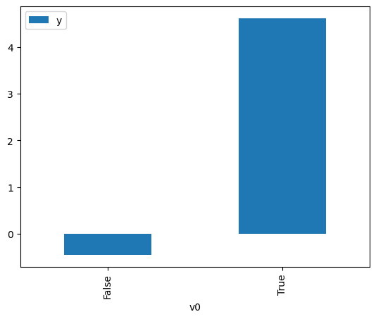
# data['df'] is just a regular pandas.DataFrame
df.causal.do(x=treatment,
             variable_types={treatment: 'b', outcome: 'c', common_cause: 'c'},
             outcome=outcome,
             common_causes=[common_cause],
            ).groupby(treatment).mean().plot(y=outcome, kind='bar')

<Axes: xlabel='v0'>

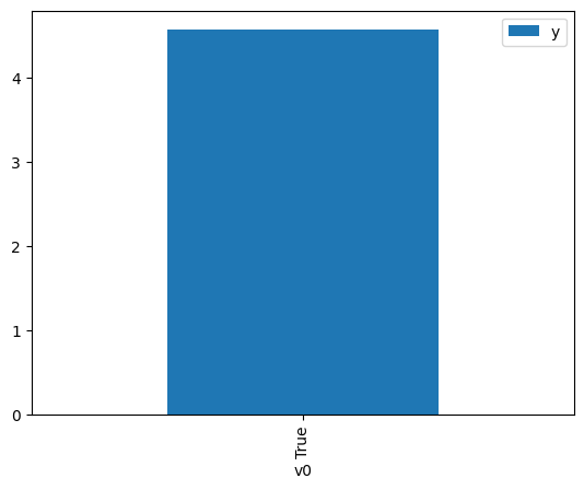
df.causal.do(x={treatment: 1},
              variable_types={treatment:'b', outcome: 'c', common_cause: 'c'},
              outcome=outcome,
              method='weighting',
              common_causes=[common_cause]
              ).groupby(treatment).mean().plot(y=outcome, kind='bar')

<Axes: xlabel='v0'>

cdf_1 = df.causal.do(x={treatment: 1},
              variable_types={treatment: 'b', outcome: 'c', common_cause: 'c'},
              outcome=outcome,
              graph=nx_graph
              )

cdf_0 = df.causal.do(x={treatment: 0},
              variable_types={treatment: 'b', outcome: 'c', common_cause: 'c'},
              outcome=outcome,
              graph=nx_graph
              )

cdf_0

	W0	v0	y	propensity_score	weight
0	-1.461199	False	-0.974013	0.859671	1.163236
1	-1.183711	False	-0.711176	0.812896	1.230169
2	-2.022528	False	-3.317512	0.924678	1.081458
3	1.225780	False	2.189129	0.180229	5.548483
4	-0.393947	False	-3.161741	0.620331	1.612041
...	...	...	...	...	...
995	-0.707376	False	0.270499	0.706632	1.415164
996	-0.728482	False	-0.762697	0.712021	1.404453
997	0.272532	False	1.806332	0.417180	2.397049
998	-1.728074	False	-0.945565	0.895017	1.117298
999	-0.797739	False	0.124563	0.729282	1.371212

1000 rows × 5 columns

cdf_1

	W0	v0	y	propensity_score	weight
0	0.160562	True	3.561945	0.548771	1.822254
1	0.110464	True	4.816448	0.533368	1.874880
2	0.673347	True	6.475563	0.696503	1.435744
3	0.407568	True	6.274436	0.622831	1.605573
4	0.736094	True	4.870072	0.712673	1.403168
...	...	...	...	...	...
995	0.437025	True	5.410330	0.631361	1.583881
996	-2.089242	True	4.667029	0.069766	14.333545
997	0.256726	True	5.886936	0.578054	1.729943
998	0.951251	True	5.494223	0.764018	1.308869
999	-1.741214	True	2.519213	0.103464	9.665161

1000 rows × 5 columns

Comparing the estimate to Linear Regression

First, estimating the effect using the causal data frame, and the 95% confidence interval.

(cdf_1['y'] - cdf_0['y']).mean()

$\displaystyle 5.10681415541703$

1.96*(cdf_1['y'] - cdf_0['y']).std() / np.sqrt(len(df))

$\displaystyle 0.125589635718884$

Comparing to the estimate from OLS.

model = OLS(np.asarray(df[outcome]), np.asarray(df[[common_cause, treatment]], dtype=np.float64))
result = model.fit()
result.summary()

OLS Regression Results

Dep. Variable:	y	R-squared (uncentered):	0.928
Model:	OLS	Adj. R-squared (uncentered):	0.928
Method:	Least Squares	F-statistic:	6411.
Date:	Sat, 08 Nov 2025	Prob (F-statistic):	0.00
Time:	05:28:06	Log-Likelihood:	-1408.9
No. Observations:	1000	AIC:	2822.
Df Residuals:	998	BIC:	2832.
Df Model:	2
Covariance Type:	nonrobust

	coef	std err	t	P>|t|	[0.025	0.975]
x1	0.9856	0.030	32.847	0.000	0.927	1.044
x2	5.0376	0.049	102.816	0.000	4.941	5.134

Omnibus:	0.277	Durbin-Watson:	1.968
Prob(Omnibus):	0.871	Jarque-Bera (JB):	0.312
Skew:	0.039	Prob(JB):	0.855
Kurtosis:	2.964	Cond. No.	1.67

Notes:
[1] R² is computed without centering (uncentered) since the model does not contain a constant.
[2] Standard Errors assume that the covariance matrix of the errors is correctly specified.