Confounding Example: Finding causal effects from observed data
Suppose you are given some data with treatment and outcome. Can you determine whether the treatment causes the outcome, or the correlation is purely due to another common cause?
[1]:
import os, sys
sys.path.append(os.path.abspath("../../../"))
[2]:
import numpy as np
import pandas as pd
import matplotlib.pyplot as plt
import math
import dowhy
from dowhy import CausalModel
import dowhy.datasets, dowhy.plotter
import logging
logging.getLogger("dowhy").setLevel(logging.WARNING)
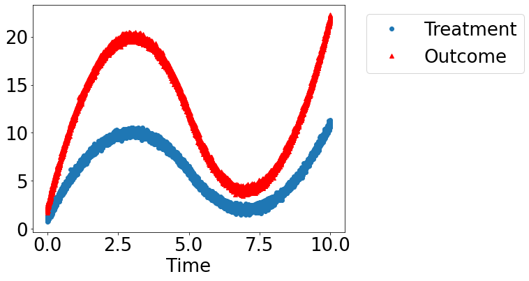
Let’s create a mystery dataset for which we need to determine whether there is a causal effect.
Creating the dataset. It is generated from either one of two models: * Model 1: Treatment does cause outcome. * Model 2: Treatment does not cause outcome. All observed correlation is due to a common cause.
[3]:
rvar = 1 if np.random.uniform() >0.5 else 0
data_dict = dowhy.datasets.xy_dataset(10000, effect=rvar,
                                      num_common_causes=1,
                                      sd_error=0.2)
df = data_dict['df']
print(df[["Treatment", "Outcome", "w0"]].head())
   Treatment    Outcome        w0
0   4.986545   9.650083 -1.139237
1   6.638307  14.064543  1.051314
2   2.396964   4.321689 -3.710417
3   7.385791  14.558907  1.427228
4   2.781060   6.330348 -2.941221
[4]:
dowhy.plotter.plot_treatment_outcome(df[data_dict["treatment_name"]], df[data_dict["outcome_name"]],
                             df[data_dict["time_val"]])
Using DoWhy to resolve the mystery: Does Treatment cause Outcome?
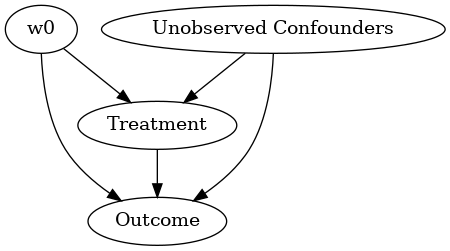
STEP 1: Model the problem as a causal graph
Initializing the causal model.
[5]:
model= CausalModel(
        data=df,
        treatment=data_dict["treatment_name"],
        outcome=data_dict["outcome_name"],
        common_causes=data_dict["common_causes_names"],
        instruments=data_dict["instrument_names"])
model.view_model(layout="dot")
WARNING:dowhy.causal_model:Causal Graph not provided. DoWhy will construct a graph based on data inputs.
Showing the causal model stored in the local file “causal_model.png”
[6]:
from IPython.display import Image, display
display(Image(filename="causal_model.png"))
STEP 2: Identify causal effect using properties of the formal causal graph
Identify the causal effect using properties of the causal graph.
[7]:
identified_estimand = model.identify_effect(proceed_when_unidentifiable=True)
print(identified_estimand)
WARNING:dowhy.causal_identifier:If this is observed data (not from a randomized experiment), there might always be missing confounders. Causal effect cannot be identified perfectly.
Estimand type: nonparametric-ate

### Estimand : 1
Estimand name: backdoor1 (Default)
Estimand expression:
     d
────────────(Expectation(Outcome|w0))
d[Treatment]
Estimand assumption 1, Unconfoundedness: If U→{Treatment} and U→Outcome then P(Outcome|Treatment,w0,U) = P(Outcome|Treatment,w0)

### Estimand : 2
Estimand name: iv
No such variable found!

### Estimand : 3
Estimand name: frontdoor
No such variable found!
STEP 3: Estimate the causal effect
Once we have identified the estimand, we can use any statistical method to estimate the causal effect.
Let’s use Linear Regression for simplicity.
[8]:
estimate = model.estimate_effect(identified_estimand,
method_name="backdoor.linear_regression")
print("Causal Estimate is " + str(estimate.value))
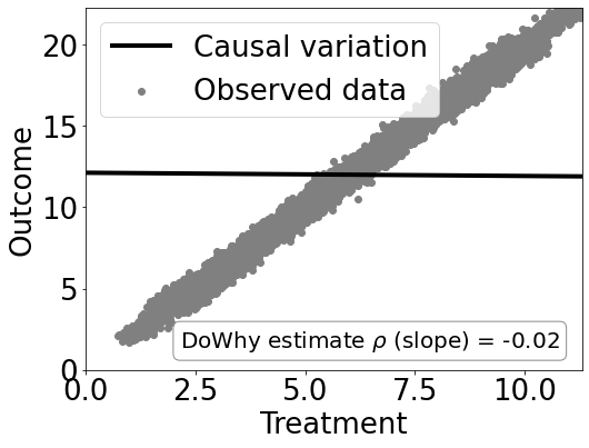
# Plot Slope of line between treamtent and outcome =causal effect
dowhy.plotter.plot_causal_effect(estimate, df[data_dict["treatment_name"]], df[data_dict["outcome_name"]])
Causal Estimate is -0.019836578259104343
Checking if the estimate is correct
[9]:
print("DoWhy estimate is " + str(estimate.value))
print ("Actual true causal effect was {0}".format(rvar))
DoWhy estimate is -0.019836578259104343
Actual true causal effect was 0
Step 4: Refuting the estimate
We can also refute the estimate to check its robustness to assumptions (aka sensitivity analysis, but on steroids).
Adding a random common cause variable
[10]:
res_random=model.refute_estimate(identified_estimand, estimate, method_name="random_common_cause")
print(res_random)
Refute: Add a Random Common Cause
Estimated effect:-0.019836578259104343
New effect:-0.019826671323794898
Replacing treatment with a random (placebo) variable
[11]:
res_placebo=model.refute_estimate(identified_estimand, estimate,
        method_name="placebo_treatment_refuter", placebo_type="permute")
print(res_placebo)
Refute: Use a Placebo Treatment
Estimated effect:-0.019836578259104343
New effect:3.341207189269113e-06
p value:0.47
Removing a random subset of the data
[12]:
res_subset=model.refute_estimate(identified_estimand, estimate,
        method_name="data_subset_refuter", subset_fraction=0.9)
print(res_subset)
Refute: Use a subset of data
Estimated effect:-0.019836578259104343
New effect:-0.019587864980808264
p value:0.47
As you can see, our causal estimator is robust to simple refutations.