Conditional Average Treatment Effects (CATE) with DoWhy and EconML
This is an experimental feature where we use EconML methods from DoWhy. Using EconML allows CATE estimation using different methods.
All four steps of causal inference in DoWhy remain the same: model, identify, estimate, and refute. The key difference is that we now call econml methods in the estimation step. There is also a simpler example using linear regression to understand the intuition behind CATE estimators.
All datasets are generated using linear structural equations.
[1]:
import numpy as np
import pandas as pd
import logging

import dowhy
from dowhy import CausalModel
import dowhy.datasets

import econml
import warnings
warnings.filterwarnings('ignore')

BETA = 10
[2]:
data = dowhy.datasets.linear_dataset(BETA, num_common_causes=4, num_samples=10000,
                                    num_instruments=2, num_effect_modifiers=2,
                                     num_treatments=1,
                                    treatment_is_binary=False,
                                    num_discrete_common_causes=2,
                                    num_discrete_effect_modifiers=0,
                                    one_hot_encode=False)
df=data['df']
print(df.head())
print("True causal estimate is", data["ate"])
         X0        X1   Z0        Z1        W0        W1 W2 W3         v0  \
0 -0.504101  0.962973  1.0  0.315426  0.689546 -2.032491  3  3  26.450136
1 -0.722767 -1.038839  0.0  0.451861 -1.006602  1.211161  3  3  18.340228
2  0.941747  0.982907  1.0  0.043433  0.827905  0.130319  3  0  22.551607
3 -0.518826  0.279882  1.0  0.703792 -2.170269  1.222133  2  2  24.344861
4  1.557961 -0.323847  1.0  0.671529 -2.630031 -0.166779  1  2  18.958443

            y
0  288.831485
1   81.064000
2  399.435222
3  214.454149
4  308.915396
True causal estimate is 13.407186604307467
[3]:
model = CausalModel(data=data["df"],
                    treatment=data["treatment_name"], outcome=data["outcome_name"],
                    graph=data["gml_graph"])
INFO:dowhy.causal_model:Model to find the causal effect of treatment ['v0'] on outcome ['y']
[4]:
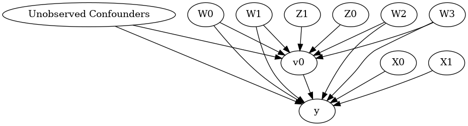
model.view_model()
from IPython.display import Image, display
display(Image(filename="causal_model.png"))
[5]:
identified_estimand= model.identify_effect(proceed_when_unidentifiable=True)
print(identified_estimand)
WARNING:dowhy.causal_identifier:If this is observed data (not from a randomized experiment), there might always be missing confounders. Causal effect cannot be identified perfectly.
INFO:dowhy.causal_identifier:Continuing by ignoring these unobserved confounders because proceed_when_unidentifiable flag is True.
INFO:dowhy.causal_identifier:Instrumental variables for treatment and outcome:['Z1', 'Z0']
INFO:dowhy.causal_identifier:Frontdoor variables for treatment and outcome:[]
Estimand type: nonparametric-ate

### Estimand : 1
Estimand name: backdoor1 (Default)
Estimand expression:
  d
─────(Expectation(y|W0,W1,W3,X1,W2,X0))
d[v₀]
Estimand assumption 1, Unconfoundedness: If U→{v0} and U→y then P(y|v0,W0,W1,W3,X1,W2,X0,U) = P(y|v0,W0,W1,W3,X1,W2,X0)

### Estimand : 2
Estimand name: backdoor2
Estimand expression:
  d
─────(Expectation(y|W0,W1,W3,X1,W2))
d[v₀]
Estimand assumption 1, Unconfoundedness: If U→{v0} and U→y then P(y|v0,W0,W1,W3,X1,W2,U) = P(y|v0,W0,W1,W3,X1,W2)

### Estimand : 3
Estimand name: backdoor3
Estimand expression:
  d
─────(Expectation(y|W0,W1,W3,W2,X0))
d[v₀]
Estimand assumption 1, Unconfoundedness: If U→{v0} and U→y then P(y|v0,W0,W1,W3,W2,X0,U) = P(y|v0,W0,W1,W3,W2,X0)

### Estimand : 4
Estimand name: backdoor4
Estimand expression:
  d
─────(Expectation(y|W0,W1,W3,W2))
d[v₀]
Estimand assumption 1, Unconfoundedness: If U→{v0} and U→y then P(y|v0,W0,W1,W3,W2,U) = P(y|v0,W0,W1,W3,W2)

### Estimand : 5
Estimand name: iv
Estimand expression:
Expectation(Derivative(y, [Z1, Z0])*Derivative([v0], [Z1, Z0])**(-1))
Estimand assumption 1, As-if-random: If U→→y then ¬(U →→{Z1,Z0})
Estimand assumption 2, Exclusion: If we remove {Z1,Z0}→{v0}, then ¬({Z1,Z0}→y)

### Estimand : 6
Estimand name: frontdoor
No such variable found!
Linear Model
First, let us build some intuition using a linear model for estimating CATE. The effect modifiers (that lead to a heterogeneous treatment effect) can be modeled as interaction terms with the treatment. Thus, their value modulates the effect of treatment.
Below the estimated effect of changing treatment from 0 to 1.
[6]:
linear_estimate = model.estimate_effect(identified_estimand,
                                        method_name="backdoor.linear_regression",
                                       control_value=0,
                                       treatment_value=1)
print(linear_estimate)
INFO:dowhy.causal_estimator:b: y~v0+W0+W1+W3+X1+W2+X0+v0*X1+v0*X0
INFO:dowhy.causal_estimator:INFO: Using Linear Regression Estimator
*** Causal Estimate ***

## Identified estimand
Estimand type: nonparametric-ate

## Realized estimand
b: y~v0+W0+W1+W3+X1+W2+X0+v0*X1+v0*X0
Target units: ate

## Estimate
Mean value: 13.407192015379287
### Conditional Estimates
__categorical__X1  __categorical__X0
(-4.035, -1.132]   (-2.529, 0.0771]      3.037913
                   (0.0771, 0.682]       6.679129
                   (0.682, 1.187]        9.361316
                   (1.187, 1.782]       11.676135
                   (1.782, 4.662]       15.723627
(-1.132, -0.54]    (-2.529, 0.0771]      5.414616
                   (0.0771, 0.682]       9.502870
                   (0.682, 1.187]       11.841804
                   (1.187, 1.782]       14.256876
                   (1.782, 4.662]       18.184712
(-0.54, -0.0227]   (-2.529, 0.0771]      7.061339
                   (0.0771, 0.682]      10.958178
                   (0.682, 1.187]       13.492511
                   (1.187, 1.782]       15.846991
                   (1.782, 4.662]       19.879993
(-0.0227, 0.55]    (-2.529, 0.0771]      8.479968
                   (0.0771, 0.682]      12.576410
                   (0.682, 1.187]       14.953556
                   (1.187, 1.782]       17.373907
                   (1.782, 4.662]       21.411765
(0.55, 3.569]      (-2.529, 0.0771]     11.157698
                   (0.0771, 0.682]      14.998151
                   (0.682, 1.187]       17.415730
                   (1.187, 1.782]       19.862391
                   (1.782, 4.662]       24.029910
dtype: float64
EconML methods
We now move to the more advanced methods from the EconML package for estimating CATE.
First, let us look at the double machine learning estimator. Method_name corresponds to the fully qualified name of the class that we want to use. For double ML, it is “econml.dml.DMLCateEstimator”.
Target units defines the units over which the causal estimate is to be computed. This can be a lambda function filter on the original dataframe, a new Pandas dataframe, or a string corresponding to the three main kinds of target units (“ate”, “att” and “atc”). Below we show an example of a lambda function.
Method_params are passed directly to EconML. For details on allowed parameters, refer to the EconML documentation.
[7]:
from sklearn.preprocessing import PolynomialFeatures
from sklearn.linear_model import LassoCV
from sklearn.ensemble import GradientBoostingRegressor
dml_estimate = model.estimate_effect(identified_estimand, method_name="backdoor.econml.dml.DML",
                                     control_value = 0,
                                     treatment_value = 1,
                                 target_units = lambda df: df["X0"]>1,  # condition used for CATE
                                 confidence_intervals=False,
                                method_params={"init_params":{'model_y':GradientBoostingRegressor(),
                                                              'model_t': GradientBoostingRegressor(),
                                                              "model_final":LassoCV(fit_intercept=False),
                                                              'featurizer':PolynomialFeatures(degree=1, include_bias=False)},
                                               "fit_params":{}})
print(dml_estimate)
INFO:dowhy.causal_estimator:INFO: Using EconML Estimator
INFO:dowhy.causal_estimator:b: y~v0+W0+W1+W3+X1+W2+X0 | X1,X0
*** Causal Estimate ***

## Identified estimand
Estimand type: nonparametric-ate

## Realized estimand
b: y~v0+W0+W1+W3+X1+W2+X0 | X1,X0
Target units: Data subset defined by a function

## Estimate
Mean value: 17.197494868852377
Effect estimates: [16.0910598  14.14293255 13.09601451 ...  7.20839431 14.33411557
 14.8303657 ]
[8]:
print("True causal estimate is", data["ate"])
True causal estimate is 13.407186604307467
[9]:
dml_estimate = model.estimate_effect(identified_estimand, method_name="backdoor.econml.dml.DML",
                                     control_value = 0,
                                     treatment_value = 1,
                                 target_units = 1,  # condition used for CATE
                                 confidence_intervals=False,
                                method_params={"init_params":{'model_y':GradientBoostingRegressor(),
                                                              'model_t': GradientBoostingRegressor(),
                                                              "model_final":LassoCV(fit_intercept=False),
                                                              'featurizer':PolynomialFeatures(degree=1, include_bias=True)},
                                               "fit_params":{}})
print(dml_estimate)
INFO:dowhy.causal_estimator:INFO: Using EconML Estimator
INFO:dowhy.causal_estimator:b: y~v0+W0+W1+W3+X1+W2+X0 | X1,X0
*** Causal Estimate ***

## Identified estimand
Estimand type: nonparametric-ate

## Realized estimand
b: y~v0+W0+W1+W3+X1+W2+X0 | X1,X0
Target units:

## Estimate
Mean value: 13.313645469650183
Effect estimates: [10.49748055  3.6845522  17.05652063 ...  0.68500175  9.12004333
 14.73724939]
CATE Object and Confidence Intervals
EconML provides its own methods to compute confidence intervals. Using BootstrapInference in the example below.
[10]:
from sklearn.preprocessing import PolynomialFeatures
from sklearn.linear_model import LassoCV
from sklearn.ensemble import GradientBoostingRegressor
from econml.inference import BootstrapInference
dml_estimate = model.estimate_effect(identified_estimand,
                                     method_name="backdoor.econml.dml.DML",
                                     target_units = "ate",
                                     confidence_intervals=True,
                                     method_params={"init_params":{'model_y':GradientBoostingRegressor(),
                                                              'model_t': GradientBoostingRegressor(),
                                                              "model_final": LassoCV(fit_intercept=False),
                                                              'featurizer':PolynomialFeatures(degree=1, include_bias=True)},
                                               "fit_params":{
                                                               'inference': BootstrapInference(n_bootstrap_samples=100, n_jobs=-1),
                                                            }
                                              })
print(dml_estimate)
INFO:dowhy.causal_estimator:INFO: Using EconML Estimator
INFO:dowhy.causal_estimator:b: y~v0+W0+W1+W3+X1+W2+X0 | X1,X0
[Parallel(n_jobs=-1)]: Using backend ThreadingBackend with 8 concurrent workers.
[Parallel(n_jobs=-1)]: Done  16 tasks      | elapsed:   30.7s
[Parallel(n_jobs=-1)]: Done 100 out of 100 | elapsed:  3.2min finished
[Parallel(n_jobs=-1)]: Using backend ThreadingBackend with 8 concurrent workers.
[Parallel(n_jobs=-1)]: Done  16 tasks      | elapsed:    0.1s
*** Causal Estimate ***

## Identified estimand
Estimand type: nonparametric-ate

## Realized estimand
b: y~v0+W0+W1+W3+X1+W2+X0 | X1,X0
Target units: ate

## Estimate
Mean value: 13.311914342959065
Effect estimates: [10.59070433  3.59638372 17.16822609 ...  0.54318894  9.03881794
 14.63167683]
95.0% confidence interval: (array([ 1.05545805e+01,  3.22946021e+00,  1.73281093e+01, ...,
       -6.49482631e-03,  8.89147258e+00,  1.45440938e+01]), array([10.9751903 ,  3.63012903, 17.69116243, ...,  0.51123116,
        9.11516389, 14.93539112]))
[Parallel(n_jobs=-1)]: Done 100 out of 100 | elapsed: 0.4s finished
Can provide a new inputs as target units and estimate CATE on them.
[11]:
test_cols= data['effect_modifier_names'] # only need effect modifiers' values
test_arr = [np.random.uniform(0,1, 10) for _ in range(len(test_cols))] # all variables are sampled uniformly, sample of 10
test_df = pd.DataFrame(np.array(test_arr).transpose(), columns=test_cols)
dml_estimate = model.estimate_effect(identified_estimand,
                                     method_name="backdoor.econml.dml.DML",
                                     target_units = test_df,
                                     confidence_intervals=False,
                                     method_params={"init_params":{'model_y':GradientBoostingRegressor(),
                                                              'model_t': GradientBoostingRegressor(),
                                                              "model_final":LassoCV(),
                                                              'featurizer':PolynomialFeatures(degree=1, include_bias=True)},
                                               "fit_params":{}
                                              })
print(dml_estimate.cate_estimates)
INFO:dowhy.causal_estimator:INFO: Using EconML Estimator
INFO:dowhy.causal_estimator:b: y~v0+W0+W1+W3+X1+W2+X0 | X1,X0
[16.53054822 12.46781996 14.48135191 12.50761403 15.52006853 13.05301137
 15.40088834 13.29661592 14.66814695 14.91607035]
Can also retrieve the raw EconML estimator object for any further operations
[12]:
print(dml_estimate._estimator_object)
<econml.dml.DML object at 0x7ff54134b2b0>
Works with any EconML method
In addition to double machine learning, below we example analyses using orthogonal forests, DRLearner (bug to fix), and neural network-based instrumental variables.
Binary treatment, Binary outcome
[13]:
data_binary = dowhy.datasets.linear_dataset(BETA, num_common_causes=4, num_samples=10000,
                                    num_instruments=2, num_effect_modifiers=2,
                                    treatment_is_binary=True, outcome_is_binary=True)
# convert boolean values to {0,1} numeric
data_binary['df'].v0 = data_binary['df'].v0.astype(int)
data_binary['df'].y = data_binary['df'].y.astype(int)
print(data_binary['df'])

model_binary = CausalModel(data=data_binary["df"],
                    treatment=data_binary["treatment_name"], outcome=data_binary["outcome_name"],
                    graph=data_binary["gml_graph"])
identified_estimand_binary = model_binary.identify_effect(proceed_when_unidentifiable=True)
INFO:dowhy.causal_model:Model to find the causal effect of treatment ['v0'] on outcome ['y']
WARNING:dowhy.causal_identifier:If this is observed data (not from a randomized experiment), there might always be missing confounders. Causal effect cannot be identified perfectly.
INFO:dowhy.causal_identifier:Continuing by ignoring these unobserved confounders because proceed_when_unidentifiable flag is True.
INFO:dowhy.causal_identifier:Instrumental variables for treatment and outcome:['Z1', 'Z0']
INFO:dowhy.causal_identifier:Frontdoor variables for treatment and outcome:[]
            X0        X1   Z0        Z1        W0        W1        W2  \
0    -0.042086 -0.807431  1.0  0.953650  0.945790 -0.200649 -2.918216
1     1.620087  0.429226  0.0  0.928747  0.188609 -1.610478 -0.057430
2    -1.575390 -1.409067  0.0  0.265052  0.469664  0.948116 -0.294454
3    -0.892651  1.103229  1.0  0.170467 -0.387164 -0.300364  0.177878
4    -0.127758  1.248801  1.0  0.076344  0.856909  0.241288  0.601427
...        ...       ...  ...       ...       ...       ...       ...
9995 -1.291579 -0.892028  0.0  0.901877 -0.660676 -0.943996  1.954166
9996 -0.961398  0.736610  0.0  0.012024 -0.188996 -1.983398 -0.331466
9997 -0.300505  0.542755  1.0  0.907418 -0.552676  0.275340 -3.810632
9998  1.358552  1.040599  1.0  0.877140 -0.253638 -0.281386 -0.649833
9999  0.167791 -0.315035  0.0  0.128057 -1.507981  0.181633  0.093358

            W3  v0  y
0     0.335050   1  1
1     0.583046   1  1
2    -0.238790   1  1
3     0.631813   1  1
4     1.705904   1  1
...        ...  .. ..
9995  0.092923   1  1
9996  0.545829   1  1
9997  1.262151   1  1
9998 -0.280275   1  1
9999  2.927231   1  1

[10000 rows x 10 columns]
Using DRLearner estimator
[14]:
from sklearn.linear_model import LogisticRegressionCV
#todo needs binary y
drlearner_estimate = model_binary.estimate_effect(identified_estimand_binary,
                                method_name="backdoor.econml.drlearner.LinearDRLearner",
                                confidence_intervals=False,
                                method_params={"init_params":{
                                                    'model_propensity': LogisticRegressionCV(cv=3, solver='lbfgs', multi_class='auto')
                                                    },
                                               "fit_params":{}
                                              })
print(drlearner_estimate)
print("True causal estimate is", data_binary["ate"])
INFO:dowhy.causal_estimator:INFO: Using EconML Estimator
INFO:dowhy.causal_estimator:b: y~v0+W0+W1+W3+X1+W2+X0 | X1,X0
*** Causal Estimate ***

## Identified estimand
Estimand type: nonparametric-ate

## Realized estimand
b: y~v0+W0+W1+W3+X1+W2+X0 | X1,X0
Target units: ate

## Estimate
Mean value: 0.5487309380359678
Effect estimates: [0.54844626 0.54665087 0.55012232 ... 0.54878221 0.54696306 0.54823195]

True causal estimate is 0.3483
Instrumental Variable Method
[15]:
import keras
from econml.deepiv import DeepIVEstimator
dims_zx = len(model._instruments)+len(model._effect_modifiers)
dims_tx = len(model._treatment)+len(model._effect_modifiers)
treatment_model = keras.Sequential([keras.layers.Dense(128, activation='relu', input_shape=(dims_zx,)), # sum of dims of Z and X
                                    keras.layers.Dropout(0.17),
                                    keras.layers.Dense(64, activation='relu'),
                                    keras.layers.Dropout(0.17),
                                    keras.layers.Dense(32, activation='relu'),
                                    keras.layers.Dropout(0.17)])
response_model = keras.Sequential([keras.layers.Dense(128, activation='relu', input_shape=(dims_tx,)), # sum of dims of T and X
                                    keras.layers.Dropout(0.17),
                                    keras.layers.Dense(64, activation='relu'),
                                    keras.layers.Dropout(0.17),
                                    keras.layers.Dense(32, activation='relu'),
                                    keras.layers.Dropout(0.17),
                                    keras.layers.Dense(1)])

deepiv_estimate = model.estimate_effect(identified_estimand,
                                        method_name="iv.econml.deepiv.DeepIV",
                                        target_units = lambda df: df["X0"]>-1,
                                        confidence_intervals=False,
                                method_params={"init_params":{'n_components': 10, # Number of gaussians in the mixture density networks
                                                              'm': lambda z, x: treatment_model(keras.layers.concatenate([z, x])), # Treatment model,
                                                              "h": lambda t, x: response_model(keras.layers.concatenate([t, x])), # Response model
                                                              'n_samples': 1, # Number of samples used to estimate the response
                                                              'first_stage_options': {'epochs':25},
                                                              'second_stage_options': {'epochs':25}
                                                             },
                                               "fit_params":{}})
print(deepiv_estimate)
Using TensorFlow backend.
INFO:dowhy.causal_estimator:INFO: Using EconML Estimator
INFO:dowhy.causal_estimator:b: y~v0+W0+W1+W3+X1+W2+X0 | X1,X0
Epoch 1/25
10000/10000 [==============================] - 3s 282us/step - loss: 8.6817
Epoch 2/25
10000/10000 [==============================] - 2s 243us/step - loss: 2.8319
Epoch 3/25
10000/10000 [==============================] - 3s 251us/step - loss: 2.5036
Epoch 4/25
10000/10000 [==============================] - 3s 263us/step - loss: 2.4126
Epoch 5/25
10000/10000 [==============================] - 2s 225us/step - loss: 2.3842
Epoch 6/25
10000/10000 [==============================] - 2s 191us/step - loss: 2.3654
Epoch 7/25
10000/10000 [==============================] - 2s 196us/step - loss: 2.3307
Epoch 8/25
10000/10000 [==============================] - 3s 263us/step - loss: 2.3166
Epoch 9/25
10000/10000 [==============================] - 3s 276us/step - loss: 2.3076
Epoch 10/25
10000/10000 [==============================] - 2s 172us/step - loss: 2.3064
Epoch 11/25
10000/10000 [==============================] - 2s 244us/step - loss: 2.2800
Epoch 12/25
10000/10000 [==============================] - 3s 257us/step - loss: 2.2787
Epoch 13/25
10000/10000 [==============================] - 2s 208us/step - loss: 2.2709
Epoch 14/25
10000/10000 [==============================] - 2s 220us/step - loss: 2.2574
Epoch 15/25
10000/10000 [==============================] - 2s 236us/step - loss: 2.2619
Epoch 16/25
10000/10000 [==============================] - 3s 253us/step - loss: 2.2484
Epoch 17/25
10000/10000 [==============================] - 3s 272us/step - loss: 2.2470
Epoch 18/25
10000/10000 [==============================] - 3s 272us/step - loss: 2.2427
Epoch 19/25
10000/10000 [==============================] - 2s 226us/step - loss: 2.2380
Epoch 20/25
10000/10000 [==============================] - 2s 183us/step - loss: 2.2262
Epoch 21/25
10000/10000 [==============================] - 2s 223us/step - loss: 2.2378
Epoch 22/25
10000/10000 [==============================] - 3s 251us/step - loss: 2.2225
Epoch 23/25
10000/10000 [==============================] - 3s 275us/step - loss: 2.2113
Epoch 24/25
10000/10000 [==============================] - 3s 256us/step - loss: 2.2175
Epoch 25/25
10000/10000 [==============================] - 2s 214us/step - loss: 2.2131
Epoch 1/25
10000/10000 [==============================] - 4s 408us/step - loss: 26474.4902
Epoch 2/25
10000/10000 [==============================] - 2s 226us/step - loss: 11620.4795
Epoch 3/25
10000/10000 [==============================] - 2s 227us/step - loss: 11070.4145
Epoch 4/25
10000/10000 [==============================] - 2s 227us/step - loss: 11041.2439
Epoch 5/25
10000/10000 [==============================] - 2s 226us/step - loss: 11187.3261
Epoch 6/25
10000/10000 [==============================] - 3s 266us/step - loss: 10696.2412
Epoch 7/25
10000/10000 [==============================] - 3s 281us/step - loss: 10785.5795
Epoch 8/25
10000/10000 [==============================] - 2s 222us/step - loss: 10922.9675
Epoch 9/25
10000/10000 [==============================] - 2s 218us/step - loss: 10585.7698
Epoch 10/25
10000/10000 [==============================] - 2s 218us/step - loss: 10826.4418
Epoch 11/25
10000/10000 [==============================] - 2s 209us/step - loss: 10643.1459
Epoch 12/25
10000/10000 [==============================] - 2s 212us/step - loss: 10495.3750
Epoch 13/25
10000/10000 [==============================] - 2s 239us/step - loss: 10615.7983
Epoch 14/25
10000/10000 [==============================] - 3s 260us/step - loss: 10692.6569
Epoch 15/25
10000/10000 [==============================] - 3s 257us/step - loss: 10604.3875
Epoch 16/25
10000/10000 [==============================] - 2s 212us/step - loss: 10558.2652
Epoch 17/25
10000/10000 [==============================] - 3s 265us/step - loss: 10516.5451
Epoch 18/25
10000/10000 [==============================] - 3s 280us/step - loss: 10710.1988
Epoch 19/25
10000/10000 [==============================] - 3s 280us/step - loss: 10746.7464
Epoch 20/25
10000/10000 [==============================] - 3s 282us/step - loss: 10653.7891
Epoch 21/25
10000/10000 [==============================] - 2s 214us/step - loss: 10314.3108
Epoch 22/25
10000/10000 [==============================] - 2s 225us/step - loss: 10651.9280
Epoch 23/25
10000/10000 [==============================] - 2s 249us/step - loss: 10478.2165
Epoch 24/25
10000/10000 [==============================] - 3s 280us/step - loss: 10524.3898
Epoch 25/25
10000/10000 [==============================] - 3s 283us/step - loss: 10680.4393
*** Causal Estimate ***

## Identified estimand
Estimand type: nonparametric-ate

### Estimand : 1
Estimand name: iv
Estimand expression:
Expectation(Derivative(y, [Z1, Z0])*Derivative([v0], [Z1, Z0])**(-1))
Estimand assumption 1, As-if-random: If U→→y then ¬(U →→{Z1,Z0})
Estimand assumption 2, Exclusion: If we remove {Z1,Z0}→{v0}, then ¬({Z1,Z0}→y)

## Realized estimand
b: y~v0+W0+W1+W3+X1+W2+X0 | X1,X0
Target units: Data subset defined by a function

## Estimate
Mean value: 5.0331292152404785
Effect estimates: [ 4.098999  -6.116501   7.234833  ...  7.00869    2.2442322  5.795349 ]
Metalearners
[16]:
data_experiment = dowhy.datasets.linear_dataset(BETA, num_common_causes=5, num_samples=10000,
                                    num_instruments=2, num_effect_modifiers=5,
                                    treatment_is_binary=True, outcome_is_binary=False)
# convert boolean values to {0,1} numeric
data_experiment['df'].v0 = data_experiment['df'].v0.astype(int)
print(data_experiment['df'])
model_experiment = CausalModel(data=data_experiment["df"],
                    treatment=data_experiment["treatment_name"], outcome=data_experiment["outcome_name"],
                    graph=data_experiment["gml_graph"])
identified_estimand_experiment = model_experiment.identify_effect(proceed_when_unidentifiable=True)
INFO:dowhy.causal_model:Model to find the causal effect of treatment ['v0'] on outcome ['y']
WARNING:dowhy.causal_identifier:If this is observed data (not from a randomized experiment), there might always be missing confounders. Causal effect cannot be identified perfectly.
INFO:dowhy.causal_identifier:Continuing by ignoring these unobserved confounders because proceed_when_unidentifiable flag is True.
INFO:dowhy.causal_identifier:Instrumental variables for treatment and outcome:['Z1', 'Z0']
INFO:dowhy.causal_identifier:Frontdoor variables for treatment and outcome:[]
            X0        X1        X2        X3        X4   Z0        Z1  \
0     1.171326 -0.064640 -0.563460  1.582340  1.756091  1.0  0.580542
1    -1.650940 -3.389096 -0.149817 -0.461226  0.219358  1.0  0.365706
2     0.765107 -0.345213 -0.738163  1.844420  1.575668  1.0  0.283551
3     0.647960 -1.742912 -0.199341  1.813745  1.681489  1.0  0.358249
4     1.348120  0.746108  0.178642  0.658514 -1.781014  1.0  0.930622
...        ...       ...       ...       ...       ...  ...       ...
9995 -0.917608  0.028557 -0.933144  1.965266  1.261264  0.0  0.341334
9996 -0.225002 -2.037790 -0.525940 -0.033352  1.699422  1.0  0.599149
9997  1.824837 -0.995047 -0.367880  1.245476 -0.721379  1.0  0.602085
9998 -0.983748 -1.956581 -1.342196  1.588319  0.285659  1.0  0.350946
9999  0.691610 -1.951029 -0.761671  0.476826 -0.353760  1.0  0.935597

            W0        W1        W2        W3        W4  v0          y
0     1.201150  1.995054  2.066612  0.753675  0.198909   1  33.512453
1    -1.268488  1.834843 -0.106924 -0.740863  1.819935   1   3.641659
2     2.010497 -1.296285  0.691936  0.636324  0.117041   1  26.831971
3    -1.262331  0.621551 -0.742102  0.711517  0.715454   1  12.701492
4     1.573959  1.537215  0.875562 -0.673198  0.455880   1  16.207716
...        ...       ...       ...       ...       ...  ..        ...
9995 -0.584633  0.701090 -0.072978  0.206021  0.234469   1  13.890869
9996 -0.007847  1.260415  0.839933  2.171979  1.856939   1  22.973153
9997  1.113284  0.190284  0.023177  0.725643 -0.294295   1  12.693518
9998  1.100263 -1.010655  2.602478  2.236147 -1.609654   1  19.194807
9999  2.677445  2.491635 -1.312530  1.555308  1.613803   1  18.246831

[10000 rows x 14 columns]
[17]:
from sklearn.ensemble import RandomForestRegressor
metalearner_estimate = model_experiment.estimate_effect(identified_estimand_experiment,
                                method_name="backdoor.econml.metalearners.TLearner",
                                confidence_intervals=False,
                                method_params={"init_params":{
                                                    'models': RandomForestRegressor()
                                                    },
                                               "fit_params":{}
                                              })
print(metalearner_estimate)
print("True causal estimate is", data_experiment["ate"])
INFO:dowhy.causal_estimator:INFO: Using EconML Estimator
WARNING:dowhy.causal_estimator:Concatenating common_causes and effect_modifiers and providing a single list of variables to metalearner estimator method, TLearner. EconML metalearners accept a single X argument.
INFO:dowhy.causal_estimator:b: y~v0+X2+X1+X3+X4+X0+W0+W1+W3+W2+W4
*** Causal Estimate ***

## Identified estimand
Estimand type: nonparametric-ate

## Realized estimand
b: y~v0+X2+X1+X3+X4+X0+W0+W1+W3+W2+W4
Target units: ate

## Estimate
Mean value: 16.94419202330739
Effect estimates: [31.04055359  9.3105599  25.82728696 ... 11.36945968 17.92448425
 19.56080328]

True causal estimate is 11.707629086241594
Refuting the estimate
Random
[18]:
res_random=model.refute_estimate(identified_estimand, dml_estimate, method_name="random_common_cause")
print(res_random)
INFO:dowhy.causal_estimator:INFO: Using EconML Estimator
INFO:dowhy.causal_estimator:b: y~v0+W0+W1+W3+X1+W2+X0 | X1,X0
Refute: Add a Random Common Cause
Estimated effect:14.284213557861628
New effect:14.257862257378136
Adding an unobserved common cause variable
[19]:
res_unobserved=model.refute_estimate(identified_estimand, dml_estimate, method_name="add_unobserved_common_cause",
                                     confounders_effect_on_treatment="linear", confounders_effect_on_outcome="linear",
                                    effect_strength_on_treatment=0.01, effect_strength_on_outcome=0.02)
print(res_unobserved)
INFO:dowhy.causal_estimator:INFO: Using EconML Estimator
INFO:dowhy.causal_estimator:b: y~v0+W0+W1+W3+X1+W2+X0 | X1,X0
Refute: Add an Unobserved Common Cause
Estimated effect:14.284213557861628
New effect:14.296399827365647
Replacing treatment with a random (placebo) variable
[20]:
res_placebo=model.refute_estimate(identified_estimand, dml_estimate,
        method_name="placebo_treatment_refuter", placebo_type="permute",
        num_simulations=10 # at least 100 is good, setting to 10 for speed
        )
print(res_placebo)
INFO:dowhy.causal_refuters.placebo_treatment_refuter:Refutation over 10 simulated datasets of permute treatment
INFO:dowhy.causal_estimator:INFO: Using EconML Estimator
INFO:dowhy.causal_estimator:b: y~placebo+W0+W1+W3+X1+W2+X0 | X1,X0
INFO:dowhy.causal_estimator:INFO: Using EconML Estimator
INFO:dowhy.causal_estimator:b: y~placebo+W0+W1+W3+X1+W2+X0 | X1,X0
INFO:dowhy.causal_estimator:INFO: Using EconML Estimator
INFO:dowhy.causal_estimator:b: y~placebo+W0+W1+W3+X1+W2+X0 | X1,X0
INFO:dowhy.causal_estimator:INFO: Using EconML Estimator
INFO:dowhy.causal_estimator:b: y~placebo+W0+W1+W3+X1+W2+X0 | X1,X0
INFO:dowhy.causal_estimator:INFO: Using EconML Estimator
INFO:dowhy.causal_estimator:b: y~placebo+W0+W1+W3+X1+W2+X0 | X1,X0
INFO:dowhy.causal_estimator:INFO: Using EconML Estimator
INFO:dowhy.causal_estimator:b: y~placebo+W0+W1+W3+X1+W2+X0 | X1,X0
INFO:dowhy.causal_estimator:INFO: Using EconML Estimator
INFO:dowhy.causal_estimator:b: y~placebo+W0+W1+W3+X1+W2+X0 | X1,X0
INFO:dowhy.causal_estimator:INFO: Using EconML Estimator
INFO:dowhy.causal_estimator:b: y~placebo+W0+W1+W3+X1+W2+X0 | X1,X0
INFO:dowhy.causal_estimator:INFO: Using EconML Estimator
INFO:dowhy.causal_estimator:b: y~placebo+W0+W1+W3+X1+W2+X0 | X1,X0
INFO:dowhy.causal_estimator:INFO: Using EconML Estimator
INFO:dowhy.causal_estimator:b: y~placebo+W0+W1+W3+X1+W2+X0 | X1,X0
WARNING:dowhy.causal_refuters.placebo_treatment_refuter:We assume a Normal Distribution as the sample has less than 100 examples.
                 Note: The underlying distribution may not be Normal. We assume that it approaches normal with the increase in sample size.
Refute: Use a Placebo Treatment
Estimated effect:14.284213557861628
New effect:-0.031152830623866274
p value:0.3458388139200408
Removing a random subset of the data
[21]:
res_subset=model.refute_estimate(identified_estimand, dml_estimate,
        method_name="data_subset_refuter", subset_fraction=0.8,
        num_simulations=10)
print(res_subset)
INFO:dowhy.causal_refuters.data_subset_refuter:Refutation over 0.8 simulated datasets of size 8000.0 each
INFO:dowhy.causal_estimator:INFO: Using EconML Estimator
INFO:dowhy.causal_estimator:b: y~v0+W0+W1+W3+X1+W2+X0 | X1,X0
INFO:dowhy.causal_estimator:INFO: Using EconML Estimator
INFO:dowhy.causal_estimator:b: y~v0+W0+W1+W3+X1+W2+X0 | X1,X0
INFO:dowhy.causal_estimator:INFO: Using EconML Estimator
INFO:dowhy.causal_estimator:b: y~v0+W0+W1+W3+X1+W2+X0 | X1,X0
INFO:dowhy.causal_estimator:INFO: Using EconML Estimator
INFO:dowhy.causal_estimator:b: y~v0+W0+W1+W3+X1+W2+X0 | X1,X0
INFO:dowhy.causal_estimator:INFO: Using EconML Estimator
INFO:dowhy.causal_estimator:b: y~v0+W0+W1+W3+X1+W2+X0 | X1,X0
INFO:dowhy.causal_estimator:INFO: Using EconML Estimator
INFO:dowhy.causal_estimator:b: y~v0+W0+W1+W3+X1+W2+X0 | X1,X0
INFO:dowhy.causal_estimator:INFO: Using EconML Estimator
INFO:dowhy.causal_estimator:b: y~v0+W0+W1+W3+X1+W2+X0 | X1,X0
INFO:dowhy.causal_estimator:INFO: Using EconML Estimator
INFO:dowhy.causal_estimator:b: y~v0+W0+W1+W3+X1+W2+X0 | X1,X0
INFO:dowhy.causal_estimator:INFO: Using EconML Estimator
INFO:dowhy.causal_estimator:b: y~v0+W0+W1+W3+X1+W2+X0 | X1,X0
INFO:dowhy.causal_estimator:INFO: Using EconML Estimator
INFO:dowhy.causal_estimator:b: y~v0+W0+W1+W3+X1+W2+X0 | X1,X0
WARNING:dowhy.causal_refuters.data_subset_refuter:We assume a Normal Distribution as the sample has less than 100 examples.
                 Note: The underlying distribution may not be Normal. We assume that it approaches normal with the increase in sample size.
Refute: Use a subset of data
Estimated effect:14.284213557861628
New effect:14.233661042403687
p value:0.17159774240261338
More refutation methods to come, especially specific to the CATE estimators.