Estimating effect of multiple treatments

import numpy as np
import pandas as pd
import logging

import dowhy
from dowhy import CausalModel
import dowhy.datasets

import econml
import warnings
warnings.filterwarnings('ignore')

data = dowhy.datasets.linear_dataset(10, num_common_causes=4, num_samples=10000,
                                    num_instruments=0, num_effect_modifiers=2,
                                     num_treatments=2,
                                    treatment_is_binary=False,
                                    num_discrete_common_causes=2,
                                    num_discrete_effect_modifiers=0,
                                    one_hot_encode=False)
df=data['df']
df.head()

	X0	X1	W0	W1	W2	W3	v0	v1	y
0	-0.413136	1.588226	0.487770	0.290617	0	0	1.133998	4.769532	79.134513
1	-1.134280	-0.198177	-1.796690	2.493473	3	1	11.873946	15.240956	-22.448157
2	-0.040000	-0.259943	0.509664	2.970383	3	0	14.436375	21.720983	178.499781
3	0.428227	-0.179278	1.130956	-1.010133	0	3	3.065979	15.740535	200.564517
4	0.879490	-0.668984	-1.299954	0.571345	3	2	8.741953	19.404153	194.187850

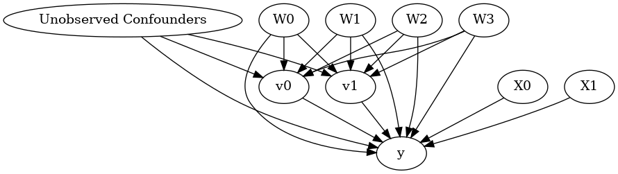
model = CausalModel(data=data["df"],
                    treatment=data["treatment_name"], outcome=data["outcome_name"],
                    graph=data["gml_graph"])

model.view_model()
from IPython.display import Image, display
display(Image(filename="causal_model.png"))

identified_estimand= model.identify_effect(proceed_when_unidentifiable=True)
print(identified_estimand)

Estimand type: nonparametric-ate

### Estimand : 1
Estimand name: backdoor
Estimand expression:
    d
─────────(Expectation(y|X1,W0,W2,W3,X0,W1))
d[v₀  v₁]
Estimand assumption 1, Unconfoundedness: If U→{v0,v1} and U→y then P(y|v0,v1,X1,W0,W2,W3,X0,W1,U) = P(y|v0,v1,X1,W0,W2,W3,X0,W1)

### Estimand : 2
Estimand name: iv
No such variable found!

### Estimand : 3
Estimand name: frontdoor
No such variable found!

Linear model

Let us first see an example for a linear model. The control_value and treatment_value can be provided as a tuple/list when the treatment is multi-dimensional.

The interpretation is change in y when v0 and v1 are changed from (0,0) to (1,1).

linear_estimate = model.estimate_effect(identified_estimand,
                                        method_name="backdoor.linear_regression",
                                       control_value=(0,0),
                                       treatment_value=(1,1),
                                       method_params={'need_conditional_estimates': False})
print(linear_estimate)

*** Causal Estimate ***

## Identified estimand
Estimand type: nonparametric-ate

### Estimand : 1
Estimand name: backdoor
Estimand expression:
    d
─────────(Expectation(y|X1,W0,W2,W3,X0,W1))
d[v₀  v₁]
Estimand assumption 1, Unconfoundedness: If U→{v0,v1} and U→y then P(y|v0,v1,X1,W0,W2,W3,X0,W1,U) = P(y|v0,v1,X1,W0,W2,W3,X0,W1)

## Realized estimand
b: y~v0+v1+X1+W0+W2+W3+X0+W1+v0*X1+v0*X0+v1*X1+v1*X0
Target units: ate

## Estimate
Mean value: 26.41126316018485

You can estimate conditional effects, based on effect modifiers.

linear_estimate = model.estimate_effect(identified_estimand,
                                        method_name="backdoor.linear_regression",
                                       control_value=(0,0),
                                       treatment_value=(1,1))
print(linear_estimate)

*** Causal Estimate ***

## Identified estimand
Estimand type: nonparametric-ate

### Estimand : 1
Estimand name: backdoor
Estimand expression:
    d
─────────(Expectation(y|X1,W0,W2,W3,X0,W1))
d[v₀  v₁]
Estimand assumption 1, Unconfoundedness: If U→{v0,v1} and U→y then P(y|v0,v1,X1,W0,W2,W3,X0,W1,U) = P(y|v0,v1,X1,W0,W2,W3,X0,W1)

## Realized estimand
b: y~v0+v1+X1+W0+W2+W3+X0+W1+v0*X1+v0*X0+v1*X1+v1*X0
Target units: ate

## Estimate
Mean value: 26.41126316018485
### Conditional Estimates
__categorical__X1  __categorical__X0
(-3.537, -1.017]   (-2.9979999999999998, 0.0335]    -52.946620
                   (0.0335, 0.628]                  -36.698335
                   (0.628, 1.109]                   -28.405206
                   (1.109, 1.706]                   -17.981903
                   (1.706, 5.283]                    -2.357185
(-1.017, -0.424]   (-2.9979999999999998, 0.0335]    -19.631323
                   (0.0335, 0.628]                   -3.214915
                   (0.628, 1.109]                     6.064157
                   (1.109, 1.706]                    15.879803
                   (1.706, 5.283]                    32.015991
(-0.424, 0.0749]   (-2.9979999999999998, 0.0335]      0.264664
                   (0.0335, 0.628]                   16.556340
                   (0.628, 1.109]                    26.187937
                   (1.109, 1.706]                    36.937134
                   (1.706, 5.283]                    52.720748
(0.0749, 0.645]    (-2.9979999999999998, 0.0335]     21.404275
                   (0.0335, 0.628]                   37.196526
                   (0.628, 1.109]                    46.502518
                   (1.109, 1.706]                    56.370240
                   (1.706, 5.283]                    72.695058
(0.645, 3.36]      (-2.9979999999999998, 0.0335]     55.298602
                   (0.0335, 0.628]                   70.148621
                   (0.628, 1.109]                    79.236172
                   (1.109, 1.706]                    89.107877
                   (1.706, 5.283]                   107.081877
dtype: float64

More methods

You can also use methods from EconML or CausalML libraries that support multiple treatments. You can look at examples from the conditional effect notebook: https://microsoft.github.io/dowhy/example_notebooks/dowhy-conditional-treatment-effects.html

Propensity-based methods do not support multiple treatments currently.