DoWhy example on the Lalonde dataset
Thanks to [@mizuy](https://github.com/mizuy) for providing this example. Here we use the Lalonde dataset and apply IPW estimator to it.
[1]:
import os, sys
sys.path.append(os.path.abspath("../../../"))

import dowhy
from dowhy import CausalModel
from rpy2.robjects import r as R
%load_ext rpy2.ipython

#%R install.packages("Matching")
%R library(Matching)
R[write to console]: Loading required package: MASS

R[write to console]: ##
##  Matching (Version 4.9-7, Build Date: 2020-02-05)
##  See http://sekhon.berkeley.edu/matching for additional documentation.
##  Please cite software as:
##   Jasjeet S. Sekhon. 2011. ``Multivariate and Propensity Score Matching
##   Software with Automated Balance Optimization: The Matching package for R.''
##   Journal of Statistical Software, 42(7): 1-52.
##
[1]:
array(['Matching', 'MASS', 'tools', 'stats', 'graphics', 'grDevices',
       'utils', 'datasets', 'methods', 'base'], dtype='<U9')
1. Load the data
[2]:
%R data(lalonde)
%R -o lalonde
lalonde = lalonde.astype({'treat':'bool'}, copy=False)
Run DoWhy analysis: model, identify, estimate
[3]:
model=CausalModel(
        data = lalonde,
        treatment='treat',
        outcome='re78',
        common_causes='nodegr+black+hisp+age+educ+married'.split('+'))
identified_estimand = model.identify_effect(proceed_when_unidentifiable=True)
estimate = model.estimate_effect(identified_estimand,
        method_name="backdoor.propensity_score_weighting",
        target_units="ate",
        method_params={"weighting_scheme":"ips_weight"})
#print(estimate)
print("Causal Estimate is " + str(estimate.value))

import statsmodels.formula.api as smf
reg=smf.wls('re78~1+treat', data=lalonde, weights=lalonde.ips_stabilized_weight)
res=reg.fit()
res.summary()
/home/amit/py-envs/env3.8/lib/python3.8/site-packages/sklearn/utils/validation.py:72: DataConversionWarning: A column-vector y was passed when a 1d array was expected. Please change the shape of y to (n_samples, ), for example using ravel().
  return f(**kwargs)
Causal Estimate is 1639.8075601428254
[3]:
| Dep. Variable: | re78 | R-squared: | 0.015 |
|---|---|---|---|
| Model: | WLS | Adj. R-squared: | 0.013 |
| Method: | Least Squares | F-statistic: | 6.743 |
| Date: | Sun, 06 Jun 2021 | Prob (F-statistic): | 0.00973 |
| Time: | 19:11:54 | Log-Likelihood: | -4544.7 |
| No. Observations: | 445 | AIC: | 9093. |
| Df Residuals: | 443 | BIC: | 9102. |
| Df Model: | 1 | ||
| Covariance Type: | nonrobust |
| coef | std err | t | P>|t| | [0.025 | 0.975] | |
|---|---|---|---|---|---|---|
| Intercept | 4555.0759 | 406.704 | 11.200 | 0.000 | 3755.767 | 5354.385 |
| treat[T.True] | 1639.8076 | 631.496 | 2.597 | 0.010 | 398.708 | 2880.907 |
| Omnibus: | 303.262 | Durbin-Watson: | 2.085 |
|---|---|---|---|
| Prob(Omnibus): | 0.000 | Jarque-Bera (JB): | 4770.581 |
| Skew: | 2.709 | Prob(JB): | 0.00 |
| Kurtosis: | 18.097 | Cond. No. | 2.47 |
Notes:
[1] Standard Errors assume that the covariance matrix of the errors is correctly specified.
Interpret the estimate
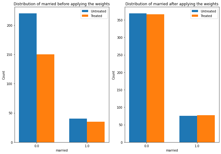
The plot below shows how the distribution of a confounder, “married” changes from the original data to the weighted data. In both datasets, we compare the distribution of “married” across treated and untreated units.
[4]:
estimate.interpret(method_name="confounder_distribution_interpreter",var_type='discrete',
                   var_name='married', fig_size = (10, 7), font_size = 12)
Sanity check: compare to manual IPW estimate
[5]:
df = model._data
ps = df['ps']
y = df['re78']
z = df['treat']

ey1 = z*y/ps / sum(z/ps)
ey0 = (1-z)*y/(1-ps) / sum((1-z)/(1-ps))
ate = ey1.sum()-ey0.sum()
print("Causal Estimate is " + str(ate))

# correct -> Causal Estimate is 1634.9868359746906
Causal Estimate is 1639.8075601428245