Confounding Example: Finding causal effects from observed data
Suppose you are given some data with treatment and outcome. Can you determine whether the treatment causes the outcome, or the correlation is purely due to another common cause?
[1]:
import os, sys
sys.path.append(os.path.abspath("../../../"))
[2]:
import numpy as np
import pandas as pd
import matplotlib.pyplot as plt
import math
import dowhy
from dowhy import CausalModel
import dowhy.datasets, dowhy.plotter
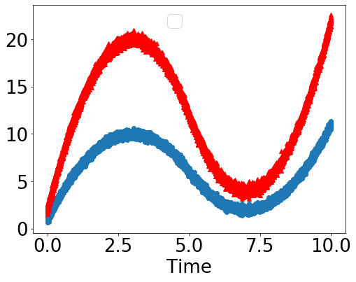
Let’s create a mystery dataset for which we need to determine whether there is a causal effect.
Creating the dataset. It is generated from either one of two models: * Model 1: Treatment does cause outcome. * Model 2: Treatment does not cause outcome. All observed correlation is due to a common cause.
[3]:
rvar = 1 if np.random.uniform() >0.5 else 0
data_dict = dowhy.datasets.xy_dataset(10000, effect=rvar, sd_error=0.2)
df = data_dict['df']
print(df[["Treatment", "Outcome", "w0"]].head())
   Treatment    Outcome        w0
0   8.329680  16.546904  2.546634
1   2.083811   4.096492 -3.995819
2   6.138014  12.041800  0.041479
3   8.874336  17.833621  2.988497
4   5.282355  10.481077 -0.860686
[4]:
dowhy.plotter.plot_treatment_outcome(df[data_dict["treatment_name"]], df[data_dict["outcome_name"]],
                             df[data_dict["time_val"]])
No handles with labels found to put in legend.
Using DoWhy to resolve the mystery: Does Treatment cause Outcome?
STEP 1: Model the problem as a causal graph
Initializing the causal model.
[5]:
model= CausalModel(
data=df,
treatment=data_dict["treatment_name"],
outcome=data_dict["outcome_name"],
common_causes=data_dict["common_causes_names"],
instruments=data_dict["instrument_names"])
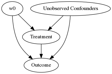
model.view_model(layout="dot")
WARNING:dowhy.causal_model:Causal Graph not provided. DoWhy will construct a graph based on data inputs.
INFO:dowhy.causal_graph:If this is observed data (not from a randomized experiment), there might always be missing confounders. Adding a node named "Unobserved Confounders" to reflect this.
INFO:dowhy.causal_model:Model to find the causal effect of treatment ['Treatment'] on outcome ['Outcome']
Showing the causal model stored in the local file “causal_model.png”
[6]:
from IPython.display import Image, display
display(Image(filename="causal_model.png"))
STEP 2: Identify causal effect using properties of the formal causal graph
Identify the causal effect using properties of the causal graph.
[7]:
identified_estimand = model.identify_effect()
print(identified_estimand)
INFO:dowhy.causal_identifier:Common causes of treatment and outcome:['w0', 'U']
WARNING:dowhy.causal_identifier:If this is observed data (not from a randomized experiment), there might always be missing confounders. Causal effect cannot be identified perfectly.
WARN: Do you want to continue by ignoring any unobserved confounders? (use proceed_when_unidentifiable=True to disable this prompt) [y/n] y
INFO:dowhy.causal_identifier:Instrumental variables for treatment and outcome:[]
Estimand type: nonparametric-ate
### Estimand : 1
Estimand name: backdoor
Estimand expression:
     d
────────────(Expectation(Outcome|w0))
d[Treatment]
Estimand assumption 1, Unconfoundedness: If U→{Treatment} and U→Outcome then P(Outcome|Treatment,w0,U) = P(Outcome|Treatment,w0)
### Estimand : 2
Estimand name: iv
No such variable found!
STEP 3: Estimate the causal effect
Once we have identified the estimand, we can use any statistical method to estimate the causal effect.
Let’s use Linear Regression for simplicity.
[8]:
estimate = model.estimate_effect(identified_estimand,
method_name="backdoor.linear_regression")
print("Causal Estimate is " + str(estimate.value))
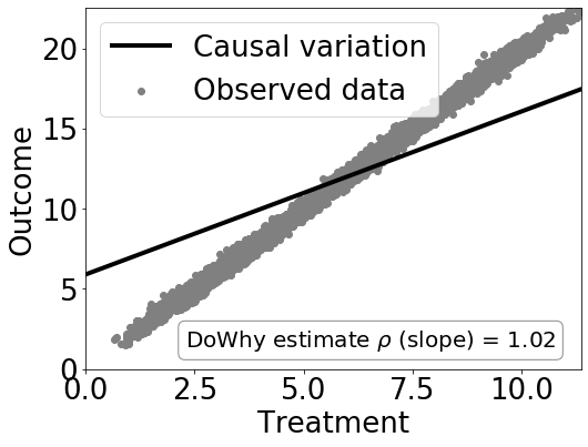
# Plot Slope of line between treamtent and outcome =causal effect
dowhy.plotter.plot_causal_effect(estimate, df[data_dict["treatment_name"]], df[data_dict["outcome_name"]])
INFO:dowhy.causal_estimator:INFO: Using Linear Regression Estimator
INFO:dowhy.causal_estimator:b: Outcome~Treatment+w0
Causal Estimate is 1.0154712956668286
Checking if the estimate is correct
[9]:
print("DoWhy estimate is " + str(estimate.value))
print ("Actual true causal effect was {0}".format(rvar))
DoWhy estimate is 1.0154712956668286
Actual true causal effect was 1
Step 4: Refuting the estimate
We can also refute the estimate to check its robustness to assumptions (aka sensitivity analysis, but on steroids).
Adding a random common cause variable
[10]:
res_random=model.refute_estimate(identified_estimand, estimate, method_name="random_common_cause")
print(res_random)
INFO:dowhy.causal_estimator:INFO: Using Linear Regression Estimator
INFO:dowhy.causal_estimator:b: Outcome~Treatment+w0+w_random
Refute: Add a Random Common Cause
Estimated effect:(1.0154712956668286,)
New effect:(1.01547620948807,)
Replacing treatment with a random (placebo) variable
[11]:
res_placebo=model.refute_estimate(identified_estimand, estimate,
        method_name="placebo_treatment_refuter", placebo_type="permute")
print(res_placebo)
INFO:dowhy.causal_estimator:INFO: Using Linear Regression Estimator
INFO:dowhy.causal_estimator:b: Outcome~placebo+w0
Refute: Use a Placebo Treatment
Estimated effect:(1.0154712956668286,)
New effect:(-0.001212143363314766,)
Removing a random subset of the data
[12]:
res_subset=model.refute_estimate(identified_estimand, estimate,
        method_name="data_subset_refuter", subset_fraction=0.9)
print(res_subset)
INFO:dowhy.causal_estimator:INFO: Using Linear Regression Estimator
INFO:dowhy.causal_estimator:b: Outcome~Treatment+w0
Refute: Use a subset of data
Estimated effect:(1.0154712956668286,)
New effect:(1.02452210674865,)
As you can see, our causal estimator is robust to simple refutations.