Conditional Average Treatment Effects (CATE) with DoWhy and EconML
This is an experimental feature where we use EconML methods from DoWhy. Using EconML allows CATE estimation using different methods.
All four steps of causal inference in DoWhy remain the same: model, identify, estimate, and refute. The key difference is that we now call econml methods in the estimation step. There is also a simpler example using linear regression to understand the intuition behind CATE estimators.
[1]:
import os, sys
sys.path.insert(1, os.path.abspath("../../../"))  # for dowhy source code
[2]:
import numpy as np
import pandas as pd
import logging

import dowhy
from dowhy import CausalModel
import dowhy.datasets

import econml
import warnings
warnings.filterwarnings('ignore')
[3]:
data = dowhy.datasets.linear_dataset(10, num_common_causes=4, num_samples=10000,
                                    num_instruments=2, num_effect_modifiers=2,
                                     num_treatments=1,
                                    treatment_is_binary=False)
df=data['df']
df.head()
[3]:
| X0 | X1 | Z0 | Z1 | W0 | W1 | W2 | W3 | v0 | y | |
|---|---|---|---|---|---|---|---|---|---|---|
| 0 | -0.423069 | -0.783912 | 1.0 | 0.595267 | -1.719039 | 1.133622 | 2.154847 | 2.093053 | 24.336479 | 168.434975 |
| 1 | -0.671984 | -0.517552 | 1.0 | 0.840097 | -0.871639 | 1.240345 | 2.513988 | 1.144102 | 32.005832 | 244.808533 |
| 2 | -0.408754 | -1.224234 | 1.0 | 0.841418 | -2.992127 | 1.947631 | 1.178079 | 0.364007 | 20.560389 | 105.083930 |
| 3 | -1.797735 | -0.810235 | 1.0 | 0.469800 | -1.097293 | -0.831213 | 0.490426 | -0.229491 | 8.713406 | 34.353637 |
| 4 | -0.579162 | -3.119641 | 1.0 | 0.691993 | -0.117981 | 0.009197 | 0.169698 | 2.553771 | 17.375187 | -28.550935 |
[4]:
model = CausalModel(data=data["df"],
                    treatment=data["treatment_name"], outcome=data["outcome_name"],
                    graph=data["gml_graph"])
INFO:dowhy.causal_model:Model to find the causal effect of treatment ['v0'] on outcome ['y']
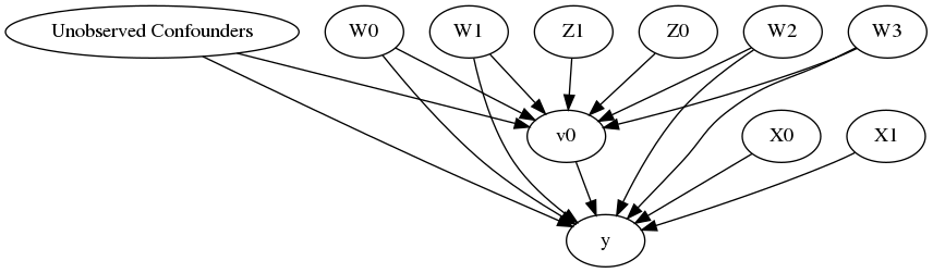
[5]:
model.view_model()
from IPython.display import Image, display
display(Image(filename="causal_model.png"))
[6]:
identified_estimand= model.identify_effect()
print(identified_estimand)
INFO:dowhy.causal_identifier:Common causes of treatment and outcome:['W0', 'W3', 'W1', 'Unobserved Confounders', 'W2']
WARNING:dowhy.causal_identifier:If this is observed data (not from a randomized experiment), there might always be missing confounders. Causal effect cannot be identified perfectly.
WARN: Do you want to continue by ignoring any unobserved confounders? (use proceed_when_unidentifiable=True to disable this prompt) [y/n] y
INFO:dowhy.causal_identifier:Instrumental variables for treatment and outcome:['Z0', 'Z1']
Estimand type: nonparametric-ate
### Estimand : 1
Estimand name: backdoor
Estimand expression:
  d
─────(Expectation(y|W0,W3,W1,W2))
d[v₀]
Estimand assumption 1, Unconfoundedness: If U→{v0} and U→y then P(y|v0,W0,W3,W1,W2,U) = P(y|v0,W0,W3,W1,W2)
### Estimand : 2
Estimand name: iv
Estimand expression:
Expectation(Derivative(y, [Z0, Z1])*Derivative([v0], [Z0, Z1])**(-1))
Estimand assumption 1, As-if-random: If U→→y then ¬(U →→{Z0,Z1})
Estimand assumption 2, Exclusion: If we remove {Z0,Z1}→{v0}, then ¬({Z0,Z1}→y)
Linear Model
First, let us build some intuition using a linear model for estimating CATE. The effect modifiers (that lead to a heterogeneous treatment effect) can be modeled as interaction terms with the treatment. Thus, their value modulates the effect of treatment.
Below the estimated effect of changing treatment from 0 to 1.
[7]:
linear_estimate = model.estimate_effect(identified_estimand,
                                        method_name="backdoor.linear_regression",
                                       control_value=0,
                                       treatment_value=1)
print(linear_estimate)
INFO:dowhy.causal_estimator:INFO: Using Linear Regression Estimator
INFO:dowhy.causal_estimator:b: y~v0+W0+W3+W1+W2+v0*X1+v0*X0
*** Causal Estimate ***

## Target estimand
Estimand type: nonparametric-ate
### Estimand : 1
Estimand name: backdoor
Estimand expression:
  d
─────(Expectation(y|W0,W3,W1,W2))
d[v₀]
Estimand assumption 1, Unconfoundedness: If U→{v0} and U→y then P(y|v0,W0,W3,W1,W2,U) = P(y|v0,W0,W3,W1,W2)
### Estimand : 2
Estimand name: iv
Estimand expression:
Expectation(Derivative(y, [Z0, Z1])*Derivative([v0], [Z0, Z1])**(-1))
Estimand assumption 1, As-if-random: If U→→y then ¬(U →→{Z0,Z1})
Estimand assumption 2, Exclusion: If we remove {Z0,Z1}→{v0}, then ¬({Z0,Z1}→y)

## Realized estimand
b: y~v0+W0+W3+W1+W2+v0*X1+v0*X0
## Estimate
Value: 10.000000000000007
EconML methods
We now move to the more advanced methods from the EconML package for estimating CATE.
First, let us look at the double machine learning estimator. Method_name corresponds to the fully qualified name of the class that we want to use. For double ML, it is “econml.dml.DMLCateEstimator”.
Target units defines the units over which the causal estimate is to be computed. This can be a lambda function filter on the original dataframe, a new Pandas dataframe, or a string corresponding to the three main kinds of target units (“ate”, “att” and “atc”). Below we show an example of a lambda function.
Method_params are passed directly to EconML. For details on allowed parameters, refer to the EconML documentation.
[8]:
from sklearn.preprocessing import PolynomialFeatures
from sklearn.linear_model import LassoCV
from sklearn.ensemble import GradientBoostingRegressor
dml_estimate = model.estimate_effect(identified_estimand, method_name="backdoor.econml.dml.DMLCateEstimator",
                                     control_value = 0,
                                     treatment_value = 1,
                                 target_units = lambda df: df["X0"]>1,  # condition used for CATE
                                 confidence_intervals=False,
                                method_params={"init_params":{'model_y':GradientBoostingRegressor(),
                                                              'model_t': GradientBoostingRegressor(),
                                                              "model_final":LassoCV(),
                                                              'featurizer':PolynomialFeatures(degree=1, include_bias=True)},
                                               "fit_params":{}})
print(dml_estimate)
INFO:dowhy.causal_estimator:INFO: Using EconML Estimator
INFO:dowhy.causal_estimator:b: y~v0+W0+W3+W1+W2
*** Causal Estimate ***

## Target estimand
Estimand type: nonparametric-ate
### Estimand : 1
Estimand name: backdoor
Estimand expression:
  d
─────(Expectation(y|W0,W3,W1,W2))
d[v₀]
Estimand assumption 1, Unconfoundedness: If U→{v0} and U→y then P(y|v0,W0,W3,W1,W2,U) = P(y|v0,W0,W3,W1,W2)
### Estimand : 2
Estimand name: iv
Estimand expression:
Expectation(Derivative(y, [Z0, Z1])*Derivative([v0], [Z0, Z1])**(-1))
Estimand assumption 1, As-if-random: If U→→y then ¬(U →→{Z0,Z1})
Estimand assumption 2, Exclusion: If we remove {Z0,Z1}→{v0}, then ¬({Z0,Z1}→y)

## Realized estimand
b: y~v0+W0+W3+W1+W2
## Estimate
Value: 8.578440374266151
[9]:
print("True causal estimate is", data["ate"])
True causal estimate is 6.531368733675461
[10]:
dml_estimate = model.estimate_effect(identified_estimand, method_name="backdoor.econml.dml.DMLCateEstimator",
                                     control_value = 0,
                                     treatment_value = 1,
                                 target_units = 1,  # condition used for CATE
                                 confidence_intervals=False,
                                method_params={"init_params":{'model_y':GradientBoostingRegressor(),
                                                              'model_t': GradientBoostingRegressor(),
                                                              "model_final":LassoCV(),
                                                              'featurizer':PolynomialFeatures(degree=1, include_bias=True)},
                                               "fit_params":{}})
print(dml_estimate)
INFO:dowhy.causal_estimator:INFO: Using EconML Estimator
INFO:dowhy.causal_estimator:b: y~v0+W0+W3+W1+W2
*** Causal Estimate ***

## Target estimand
Estimand type: nonparametric-ate
### Estimand : 1
Estimand name: backdoor
Estimand expression:
  d
─────(Expectation(y|W0,W3,W1,W2))
d[v₀]
Estimand assumption 1, Unconfoundedness: If U→{v0} and U→y then P(y|v0,W0,W3,W1,W2,U) = P(y|v0,W0,W3,W1,W2)
### Estimand : 2
Estimand name: iv
Estimand expression:
Expectation(Derivative(y, [Z0, Z1])*Derivative([v0], [Z0, Z1])**(-1))
Estimand assumption 1, As-if-random: If U→→y then ¬(U →→{Z0,Z1})
Estimand assumption 2, Exclusion: If we remove {Z0,Z1}→{v0}, then ¬({Z0,Z1}→y)

## Realized estimand
b: y~v0+W0+W3+W1+W2
## Estimate
Value: 6.478668642785378
CATE Object and Confidence Intervals
[11]:
from sklearn.preprocessing import PolynomialFeatures
from sklearn.linear_model import LassoCV
from sklearn.ensemble import GradientBoostingRegressor
dml_estimate = model.estimate_effect(identified_estimand,
                                     method_name="backdoor.econml.dml.DMLCateEstimator",
                                     target_units = lambda df: df["X0"]>1,
                                     confidence_intervals=True,
                                     method_params={"init_params":{'model_y':GradientBoostingRegressor(),
                                                              'model_t': GradientBoostingRegressor(),
                                                              "model_final":LassoCV(),
                                                              'featurizer':PolynomialFeatures(degree=1, include_bias=True)},
                                               "fit_params":{
                                                               'inference': 'bootstrap',
                                                            }
                                              })
print(dml_estimate)
print(dml_estimate.cate_estimates[:10])
print(dml_estimate.effect_intervals)
INFO:dowhy.causal_estimator:INFO: Using EconML Estimator
INFO:dowhy.causal_estimator:b: y~v0+W0+W3+W1+W2
[Parallel(n_jobs=-1)]: Using backend ThreadingBackend with 32 concurrent workers.
[Parallel(n_jobs=-1)]: Done  71 out of 100 | elapsed:  1.1min remaining:   27.4s
[Parallel(n_jobs=-1)]: Done 100 out of 100 | elapsed:  1.2min finished
[Parallel(n_jobs=-1)]: Using backend ThreadingBackend with 32 concurrent workers.
*** Causal Estimate ***

## Target estimand
Estimand type: nonparametric-ate
### Estimand : 1
Estimand name: backdoor
Estimand expression:
  d
─────(Expectation(y|W0,W3,W1,W2))
d[v₀]
Estimand assumption 1, Unconfoundedness: If U→{v0} and U→y then P(y|v0,W0,W3,W1,W2,U) = P(y|v0,W0,W3,W1,W2)
### Estimand : 2
Estimand name: iv
Estimand expression:
Expectation(Derivative(y, [Z0, Z1])*Derivative([v0], [Z0, Z1])**(-1))
Estimand assumption 1, As-if-random: If U→→y then ¬(U →→{Z0,Z1})
Estimand assumption 2, Exclusion: If we remove {Z0,Z1}→{v0}, then ¬({Z0,Z1}→y)

## Realized estimand
b: y~v0+W0+W3+W1+W2
## Estimate
Value: 8.59526782752452

[[11.26396103]
 [10.54322021]
 [ 8.16997949]
 [ 4.86061276]
 [11.09707173]
 [-2.36778738]
 [ 4.65848744]
 [ 6.6349523 ]
 [ 7.01785881]
 [ 9.61921864]]
(array([[10.7209148 ],
       [10.05703784],
       [ 7.82636093],
       ...,
       [10.37314163],
       [ 5.89648783],
       [14.28637593]]), array([[10.98146476],
       [10.28543916],
       [ 8.04793421],
       ...,
       [10.63228411],
       [ 6.08169175],
       [14.69742395]]))
[Parallel(n_jobs=-1)]: Done  71 out of 100 | elapsed:    0.1s remaining:    0.0s
[Parallel(n_jobs=-1)]: Done 100 out of 100 | elapsed:    0.1s finished
Can provide a new inputs as target units and estimate CATE on them.
[12]:
test_cols= data['effect_modifier_names'] # only need effect modifiers' values
test_arr = [np.random.uniform(0,1, 10) for _ in range(len(test_cols))] # all variables are sampled uniformly, sample of 10
test_df = pd.DataFrame(np.array(test_arr).transpose(), columns=test_cols)
dml_estimate = model.estimate_effect(identified_estimand,
                                     method_name="backdoor.econml.dml.DMLCateEstimator",
                                     target_units = test_df,
                                     confidence_intervals=False,
                                     method_params={"init_params":{'model_y':GradientBoostingRegressor(),
                                                              'model_t': GradientBoostingRegressor(),
                                                              "model_final":LassoCV(),
                                                              'featurizer':PolynomialFeatures(degree=1, include_bias=True)},
                                               "fit_params":{}
                                              })
print(dml_estimate.cate_estimates)
INFO:dowhy.causal_estimator:INFO: Using EconML Estimator
INFO:dowhy.causal_estimator:b: y~v0+W0+W3+W1+W2
[[10.98805765]
 [13.07006079]
 [10.63717349]
 [11.88142705]
 [12.24428257]
 [14.27632508]
 [13.19014829]
 [11.06457798]
 [11.51427196]
 [12.50204303]]
Can also retrieve the raw EconML estimator object for any further operations
[13]:
print(dml_estimate._estimator_object)
dml_estimate
<econml.dml.DMLCateEstimator object at 0x7fff577ce940>
[13]:
<dowhy.causal_estimator.CausalEstimate at 0x7fff577ce828>
Works with any EconML method
In addition to double machine learning, below we example analyses using orthogonal forests, DRLearner (bug to fix), and neural network-based instrumental variables.
Continuous treatment, Continuous outcome
[14]:
from sklearn.linear_model import LogisticRegression
orthoforest_estimate = model.estimate_effect(identified_estimand, method_name="backdoor.econml.ortho_forest.ContinuousTreatmentOrthoForest",
                                 target_units = lambda df: df["X0"]>1,
                                 confidence_intervals=False,
                                method_params={"init_params":{
                                                    'n_trees':2, # not ideal, just as an example to speed up computation
                                                    },
                                               "fit_params":{}
                                              })
print(orthoforest_estimate)
INFO:dowhy.causal_estimator:INFO: Using EconML Estimator
INFO:dowhy.causal_estimator:b: y~v0+W0+W3+W1+W2
[Parallel(n_jobs=-1)]: Using backend LokyBackend with 32 concurrent workers.
[Parallel(n_jobs=-1)]: Done   2 out of   2 | elapsed:   38.9s remaining:    0.0s
[Parallel(n_jobs=-1)]: Done   2 out of   2 | elapsed:   38.9s finished
[Parallel(n_jobs=-1)]: Using backend LokyBackend with 32 concurrent workers.
[Parallel(n_jobs=-1)]: Done   2 out of   2 | elapsed:   11.7s remaining:    0.0s
[Parallel(n_jobs=-1)]: Done   2 out of   2 | elapsed:   11.7s finished
[Parallel(n_jobs=-1)]: Using backend ThreadingBackend with 32 concurrent workers.
[Parallel(n_jobs=-1)]: Done  64 tasks      | elapsed:   34.5s
[Parallel(n_jobs=-1)]: Done 224 tasks      | elapsed:  1.7min
[Parallel(n_jobs=-1)]: Done 448 tasks      | elapsed:  3.5min
[Parallel(n_jobs=-1)]: Done 736 tasks      | elapsed:  5.8min
[Parallel(n_jobs=-1)]: Done 1088 tasks      | elapsed:  8.6min
*** Causal Estimate ***

## Target estimand
Estimand type: nonparametric-ate
### Estimand : 1
Estimand name: backdoor
Estimand expression:
  d
─────(Expectation(y|W0,W3,W1,W2))
d[v₀]
Estimand assumption 1, Unconfoundedness: If U→{v0} and U→y then P(y|v0,W0,W3,W1,W2,U) = P(y|v0,W0,W3,W1,W2)
### Estimand : 2
Estimand name: iv
Estimand expression:
Expectation(Derivative(y, [Z0, Z1])*Derivative([v0], [Z0, Z1])**(-1))
Estimand assumption 1, As-if-random: If U→→y then ¬(U →→{Z0,Z1})
Estimand assumption 2, Exclusion: If we remove {Z0,Z1}→{v0}, then ¬({Z0,Z1}→y)

## Realized estimand
b: y~v0+W0+W3+W1+W2
## Estimate
Value: 8.331353134942322
[Parallel(n_jobs=-1)]: Done 1483 out of 1483 | elapsed: 11.6min finished
Binary treatment, Binary outcome
[15]:
data_binary = dowhy.datasets.linear_dataset(10, num_common_causes=4, num_samples=10000,
                                    num_instruments=2, num_effect_modifiers=2,
                                    treatment_is_binary=True, outcome_is_binary=True)
print(data_binary['df'])

model_binary = CausalModel(data=data_binary["df"],
                    treatment=data_binary["treatment_name"], outcome=data_binary["outcome_name"],
                    graph=data_binary["gml_graph"])
identified_estimand_binary = model_binary.identify_effect(proceed_when_unidentifiable=True)
INFO:dowhy.causal_model:Model to find the causal effect of treatment ['v0'] on outcome ['y']
INFO:dowhy.causal_identifier:Common causes of treatment and outcome:['W0', 'W3', 'W1', 'Unobserved Confounders', 'W2']
WARNING:dowhy.causal_identifier:If this is observed data (not from a randomized experiment), there might always be missing confounders. Causal effect cannot be identified perfectly.
INFO:dowhy.causal_identifier:Continuing by ignoring these unobserved confounders because proceed_when_unidentifiable flag is True.
INFO:dowhy.causal_identifier:Instrumental variables for treatment and outcome:['Z0', 'Z1']
            X0        X1   Z0        Z1        W0        W1        W2  \
0     1.170983 -0.463676  0.0  0.999261  1.265824 -0.591487  0.187607
1     1.874968 -1.237442  0.0  0.372351  2.055680 -0.470702 -1.089608
2    -0.231365  0.227272  0.0  0.517914  1.004229 -1.196373 -2.495002
3     1.313117  0.065614  0.0  0.793337 -0.316458 -0.459159 -0.455055
4     0.012586  0.194818  0.0  0.683885 -0.322924 -1.523299 -0.816566
...        ...       ...  ...       ...       ...       ...       ...
9995  2.170496 -0.544734  0.0  0.251869  0.903261 -1.776711 -0.312277
9996  0.359327  0.190037  0.0  0.877978  1.832255 -1.413621 -1.064130
9997 -0.515581 -2.971678  0.0  0.482088  0.136553  0.119679  0.081736
9998  0.105968 -1.541644  0.0  0.095357  3.035971 -1.195416 -0.069832
9999  1.180787 -0.944992  0.0  0.265338  0.176723  1.442231 -1.669103

            W3     v0      y
0     0.281102   True   True
1    -0.175620   True  False
2    -1.024748  False   True
3     2.365471   True  False
4    -1.955707  False   True
...        ...    ...    ...
9995 -0.112627  False   True
9996 -2.130779   True   True
9997 -0.567688   True   True
9998  0.280326   True  False
9999 -0.242490   True   True

[10000 rows x 10 columns]
NOTE: DRLearner throws an error since it expects the outcome in a 1-D array. This will be fixed soon in the EconML package.
[17]:
from sklearn.linear_model import LogisticRegressionCV
#todo needs binary y
drlearner_estimate = model_binary.estimate_effect(identified_estimand_binary,
                                method_name="backdoor.econml.drlearner.LinearDRLearner",
                                target_units = lambda df: df["X0"]>1,
                                confidence_intervals=False,
                                method_params={"init_params":{
                                                    'model_propensity': LogisticRegressionCV(cv=3, solver='lbfgs', multi_class='auto')
                                                    },
                                               "fit_params":{}
                                              })
print(drlearner_estimate)
INFO:dowhy.causal_estimator:INFO: Using EconML Estimator
INFO:dowhy.causal_estimator:b: y~v0+W0+W3+W1+W2
---------------------------------------------------------------------------
AssertionError                            Traceback (most recent call last)
<ipython-input-17-f77b6b495b1d> in <module>
      8                                                     'model_propensity': LogisticRegressionCV(cv=3, solver='lbfgs', multi_class='auto')
      9                                                     },
---> 10                                                "fit_params":{}
     11                                               })
     12 print(drlearner_estimate)

/mnt/c/Users/amshar/code/dowhy/dowhy/causal_model.py in estimate_effect(self, identified_estimand, method_name, control_value, treatment_value, test_significance, evaluate_effect_strength, confidence_intervals, target_units, effect_modifiers, method_params)
    205                 params=method_params
    206             )
--> 207             estimate = causal_estimator.estimate_effect()
    208             # Store parameters inside estimate object for refutation methods
    209             estimate.add_params(

/mnt/c/Users/amshar/code/dowhy/dowhy/causal_estimator.py in estimate_effect(self)
     88         """
     89
---> 90         est = self._estimate_effect()
     91         self._estimate = est
     92

/mnt/c/Users/amshar/code/dowhy/dowhy/causal_estimators/econml_cate_estimator.py in _estimate_effect(self)
     66         # Calling the econml estimator's fit method
     67         if self.identifier_method == "backdoor":
---> 68             self.estimator.fit(Y, T, X, W, **self.method_params["fit_params"])
     69         else:
     70             self.estimator.fit(Y, T, X, Z, **self.method_params["fit_params"])

~/python-environments/vpy36/lib/python3.6/site-packages/econml/drlearner.py in fit(self, Y, T, X, W, sample_weight, sample_var, inference)
    656         """
    657         # Replacing fit from DRLearner, to add statsmodels inference in docstring
--> 658         return super().fit(Y, T, X=X, W=W, sample_weight=sample_weight, sample_var=sample_var, inference=inference)
    659
    660     @property

~/python-environments/vpy36/lib/python3.6/site-packages/econml/drlearner.py in fit(self, Y, T, X, W, sample_weight, sample_var, inference)
    364         """
    365         # Replacing fit from _OrthoLearner, to enforce Z=None and improve the docstring
--> 366         return super().fit(Y, T, X=X, W=W, sample_weight=sample_weight, sample_var=sample_var, inference=inference)
    367
    368     def score(self, Y, T, X=None, W=None):

~/python-environments/vpy36/lib/python3.6/site-packages/econml/cate_estimator.py in call(self, Y, T, inference, *args, **kwargs)
     87                 inference.prefit(self, Y, T, *args, **kwargs)
     88             # call the wrapped fit method
---> 89             m(self, Y, T, *args, **kwargs)
     90             if inference is not None:
     91                 # NOTE: we call inference fit *after* calling the main fit method

~/python-environments/vpy36/lib/python3.6/site-packages/econml/_ortho_learner.py in fit(self, Y, T, X, W, Z, sample_weight, sample_var, inference)
    478         """
    479         self._check_input_dims(Y, T, X, W, Z, sample_weight, sample_var)
--> 480         nuisances, fitted_inds = self._fit_nuisances(Y, T, X, W, Z, sample_weight=sample_weight)
    481         self._fit_final(self._subinds_check_none(Y, fitted_inds),
    482                         self._subinds_check_none(T, fitted_inds),

~/python-environments/vpy36/lib/python3.6/site-packages/econml/_ortho_learner.py in _fit_nuisances(self, Y, T, X, W, Z, sample_weight)
    516
    517         nuisances, fitted_models, fitted_inds = _crossfit(self._model_nuisance, folds,
--> 518                                                           Y, T, X=X, W=W, Z=Z, sample_weight=sample_weight)
    519         self._models_nuisance = fitted_models
    520         return nuisances, fitted_inds

~/python-environments/vpy36/lib/python3.6/site-packages/econml/_ortho_learner.py in _crossfit(model, folds, *args, **kwargs)
    143                 kwargs_test[key] = var[test_idxs]
    144
--> 145         model_list[idx].fit(*args_train, **kwargs_train)
    146
    147         nuisance_temp = model_list[idx].predict(*args_test, **kwargs_test)

~/python-environments/vpy36/lib/python3.6/site-packages/econml/drlearner.py in fit(self, Y, T, X, W, sample_weight)
    260             def fit(self, Y, T, X=None, W=None, *, sample_weight=None):
    261                 # TODO Allow for non-vector y, i.e. of shape (n, 1)
--> 262                 assert np.ndim(Y) == 1, "Can only accept single dimensional outcomes Y! Use Y.ravel()."
    263                 if (X is None) and (W is None):
    264                     raise AttributeError("At least one of X or W has to not be None!")

AssertionError: Can only accept single dimensional outcomes Y! Use Y.ravel().
Instrumental Variable Method
[18]:
import keras
from econml.deepiv import DeepIVEstimator
dims_zx = len(model._instruments)+len(model._effect_modifiers)
dims_tx = len(model._treatment)+len(model._effect_modifiers)
treatment_model = keras.Sequential([keras.layers.Dense(128, activation='relu', input_shape=(dims_zx,)), # sum of dims of Z and X
                                    keras.layers.Dropout(0.17),
                                    keras.layers.Dense(64, activation='relu'),
                                    keras.layers.Dropout(0.17),
                                    keras.layers.Dense(32, activation='relu'),
                                    keras.layers.Dropout(0.17)])
response_model = keras.Sequential([keras.layers.Dense(128, activation='relu', input_shape=(dims_tx,)), # sum of dims of T and X
                                    keras.layers.Dropout(0.17),
                                    keras.layers.Dense(64, activation='relu'),
                                    keras.layers.Dropout(0.17),
                                    keras.layers.Dense(32, activation='relu'),
                                    keras.layers.Dropout(0.17),
                                    keras.layers.Dense(1)])

deepiv_estimate = model.estimate_effect(identified_estimand,
                                        method_name="iv.econml.deepiv.DeepIVEstimator",
                                        target_units = lambda df: df["X0"]>-1,
                                        confidence_intervals=False,
                                method_params={"init_params":{'n_components': 10, # Number of gaussians in the mixture density networks
                                                              'm': lambda z, x: treatment_model(keras.layers.concatenate([z, x])), # Treatment model,
                                                              "h": lambda t, x: response_model(keras.layers.concatenate([t, x])), # Response model
                                                              'n_samples': 1, # Number of samples used to estimate the response
                                                              'first_stage_options': {'epochs':25},
                                                              'second_stage_options': {'epochs':25}
                                                             },
                                               "fit_params":{}})
print(deepiv_estimate)
Using TensorFlow backend.
INFO:dowhy.causal_estimator:INFO: Using EconML Estimator
INFO:dowhy.causal_estimator:b: y~v0+W0+W3+W1+W2
WARNING:tensorflow:From /home/amshar/python-environments/vpy36/lib/python3.6/site-packages/tensorflow/python/ops/math_ops.py:2403: add_dispatch_support.<locals>.wrapper (from tensorflow.python.ops.array_ops) is deprecated and will be removed in a future version.
Instructions for updating:
Use tf.where in 2.0, which has the same broadcast rule as np.where
WARNING:tensorflow:From /home/amshar/python-environments/vpy36/lib/python3.6/site-packages/keras/backend/tensorflow_backend.py:422: The name tf.global_variables is deprecated. Please use tf.compat.v1.global_variables instead.
Epoch 1/25
10000/10000 [==============================] - 1s 125us/step - loss: 5.7914
Epoch 2/25
10000/10000 [==============================] - 1s 69us/step - loss: 2.7293
Epoch 3/25
10000/10000 [==============================] - 1s 67us/step - loss: 2.5698
Epoch 4/25
10000/10000 [==============================] - 1s 67us/step - loss: 2.5207
Epoch 5/25
10000/10000 [==============================] - 1s 67us/step - loss: 2.4888
Epoch 6/25
10000/10000 [==============================] - 1s 66us/step - loss: 2.4770
Epoch 7/25
10000/10000 [==============================] - 1s 67us/step - loss: 2.4734
Epoch 8/25
10000/10000 [==============================] - 1s 66us/step - loss: 2.4526
Epoch 9/25
10000/10000 [==============================] - 1s 67us/step - loss: 2.4543
Epoch 10/25
10000/10000 [==============================] - 1s 67us/step - loss: 2.4469
Epoch 11/25
10000/10000 [==============================] - 1s 67us/step - loss: 2.4347
Epoch 12/25
10000/10000 [==============================] - 1s 67us/step - loss: 2.4246
Epoch 13/25
10000/10000 [==============================] - 1s 67us/step - loss: 2.4259
Epoch 14/25
10000/10000 [==============================] - 1s 66us/step - loss: 2.4241
Epoch 15/25
10000/10000 [==============================] - 1s 66us/step - loss: 2.4149
Epoch 16/25
10000/10000 [==============================] - 1s 66us/step - loss: 2.4150
Epoch 17/25
10000/10000 [==============================] - 1s 66us/step - loss: 2.4078
Epoch 18/25
10000/10000 [==============================] - 1s 66us/step - loss: 2.4015
Epoch 19/25
10000/10000 [==============================] - 1s 67us/step - loss: 2.4001
Epoch 20/25
10000/10000 [==============================] - 1s 67us/step - loss: 2.4029
Epoch 21/25
10000/10000 [==============================] - 1s 67us/step - loss: 2.4025
Epoch 22/25
10000/10000 [==============================] - 1s 66us/step - loss: 2.3970
Epoch 23/25
10000/10000 [==============================] - 1s 66us/step - loss: 2.3930
Epoch 24/25
10000/10000 [==============================] - 1s 66us/step - loss: 2.3982
Epoch 25/25
10000/10000 [==============================] - 1s 66us/step - loss: 2.3940
Epoch 1/25
10000/10000 [==============================] - 2s 205us/step - loss: 8526.7076
Epoch 2/25
10000/10000 [==============================] - 1s 111us/step - loss: 4659.4835
Epoch 3/25
10000/10000 [==============================] - 1s 107us/step - loss: 4231.5569
Epoch 4/25
10000/10000 [==============================] - 1s 104us/step - loss: 4215.2266
Epoch 5/25
10000/10000 [==============================] - 1s 102us/step - loss: 4090.3670
Epoch 6/25
10000/10000 [==============================] - 1s 102us/step - loss: 4030.0446
Epoch 7/25
10000/10000 [==============================] - 1s 100us/step - loss: 4137.3973
Epoch 8/25
10000/10000 [==============================] - 1s 98us/step - loss: 4091.2221
Epoch 9/25
10000/10000 [==============================] - 1s 97us/step - loss: 4003.9576
Epoch 10/25
10000/10000 [==============================] - 1s 97us/step - loss: 4013.2564
Epoch 11/25
10000/10000 [==============================] - 1s 98us/step - loss: 4035.7388
Epoch 12/25
10000/10000 [==============================] - 1s 97us/step - loss: 3965.2224
Epoch 13/25
10000/10000 [==============================] - 1s 98us/step - loss: 4054.5777
Epoch 14/25
10000/10000 [==============================] - 1s 97us/step - loss: 4014.5290
Epoch 15/25
10000/10000 [==============================] - 1s 97us/step - loss: 3984.4700
Epoch 16/25
10000/10000 [==============================] - 1s 96us/step - loss: 3926.2307
Epoch 17/25
10000/10000 [==============================] - 1s 94us/step - loss: 4015.3016
Epoch 18/25
10000/10000 [==============================] - 1s 94us/step - loss: 4034.1578
Epoch 19/25
10000/10000 [==============================] - 1s 94us/step - loss: 3974.5770
Epoch 20/25
10000/10000 [==============================] - 1s 94us/step - loss: 3985.2165
Epoch 21/25
10000/10000 [==============================] - 1s 94us/step - loss: 3977.9142
Epoch 22/25
10000/10000 [==============================] - 1s 94us/step - loss: 3950.7200
Epoch 23/25
10000/10000 [==============================] - 1s 94us/step - loss: 4011.0488
Epoch 24/25
10000/10000 [==============================] - 1s 93us/step - loss: 3986.2898
Epoch 25/25
10000/10000 [==============================] - 1s 94us/step - loss: 4029.8864
*** Causal Estimate ***

## Target estimand
Estimand type: nonparametric-ate
### Estimand : 1
Estimand name: backdoor
Estimand expression:
  d
─────(Expectation(y|W0,W3,W1,W2))
d[v₀]
Estimand assumption 1, Unconfoundedness: If U→{v0} and U→y then P(y|v0,W0,W3,W1,W2,U) = P(y|v0,W0,W3,W1,W2)
### Estimand : 2
Estimand name: iv
Estimand expression:
Expectation(Derivative(y, [Z0, Z1])*Derivative([v0], [Z0, Z1])**(-1))
Estimand assumption 1, As-if-random: If U→→y then ¬(U →→{Z0,Z1})
Estimand assumption 2, Exclusion: If we remove {Z0,Z1}→{v0}, then ¬({Z0,Z1}→y)

## Realized estimand
b: y~v0+W0+W3+W1+W2
## Estimate
Value: 6.484096527099609
Refuting the estimate
Random
[19]:
res_random=model.refute_estimate(identified_estimand, dml_estimate, method_name="random_common_cause")
print(res_random)
INFO:dowhy.causal_estimator:INFO: Using EconML Estimator
INFO:dowhy.causal_estimator:b: y~v0+W0+W3+W1+W2+w_random
Refute: Add a Random Common Cause
Estimated effect:(12.13683678878986,)
New effect:(13.248034250593435,)
Adding an unobserved common cause variable
[20]:
res_unobserved=model.refute_estimate(identified_estimand, dml_estimate, method_name="add_unobserved_common_cause",
                                     confounders_effect_on_treatment="linear", confounders_effect_on_outcome="linear",
                                    effect_strength_on_treatment=0.01, effect_strength_on_outcome=0.02)
print(res_unobserved)
INFO:dowhy.causal_estimator:INFO: Using EconML Estimator
INFO:dowhy.causal_estimator:b: y~v0+W0+W3+W1+W2
Refute: Add an Unobserved Common Cause
Estimated effect:(12.13683678878986,)
New effect:(13.196059198878597,)
Replacing treatment with a random (placebo) variable
[21]:
res_placebo=model.refute_estimate(identified_estimand, dml_estimate,
        method_name="placebo_treatment_refuter", placebo_type="permute")
print(res_placebo)
INFO:dowhy.causal_estimator:INFO: Using EconML Estimator
INFO:dowhy.causal_estimator:b: y~placebo+W0+W3+W1+W2
Refute: Use a Placebo Treatment
Estimated effect:(12.13683678878986,)
New effect:(0.0,)
Removing a random subset of the data
[22]:
res_subset=model.refute_estimate(identified_estimand, dml_estimate,
        method_name="data_subset_refuter", subset_fraction=0.8)
print(res_subset)
INFO:dowhy.causal_estimator:INFO: Using EconML Estimator
INFO:dowhy.causal_estimator:b: y~v0+W0+W3+W1+W2
Refute: Use a subset of data
Estimated effect:(12.13683678878986,)
New effect:(13.150007335670214,)
More refutation methods to come, especially specific to the CATE estimators.