Demo for the DoWhy causal API
We show a simple example of adding a causal extension to any dataframe.
[1]:
import os, sys
sys.path.append(os.path.abspath("../../../"))
[2]:
import dowhy.datasets
import dowhy.api

import numpy as np
import pandas as pd

from statsmodels.api import OLS
[3]:
data = dowhy.datasets.linear_dataset(beta=5,
        num_common_causes=1,
        num_instruments = 0,
        num_samples=1000,
        treatment_is_binary=True)
df = data['df']
df['y'] = df['y'] + np.random.normal(size=len(df)) # Adding noise to data. Without noise, the variance in Y|X, Z is zero, and mcmc fails.
#data['dot_graph'] = 'digraph { v ->y;X0-> v;X0-> y;}'

treatment= data["treatment_name"][0]
outcome = data["outcome_name"][0]
common_cause = data["common_causes_names"][0]
df
[3]:
| W0 | v0 | y | |
|---|---|---|---|
| 0 | 0.230046 | False | 0.328777 |
| 1 | -0.625509 | True | 3.794958 |
| 2 | -2.600417 | False | -5.214096 |
| 3 | 0.146942 | False | 1.361876 |
| 4 | -0.919551 | False | -2.228864 |
| ... | ... | ... | ... |
| 995 | -0.063647 | False | 0.117779 |
| 996 | -1.962547 | False | -4.034488 |
| 997 | -0.089728 | True | 5.780041 |
| 998 | -0.334302 | True | 3.872871 |
| 999 | -2.410448 | False | -4.524930 |
1000 rows × 3 columns
[4]:
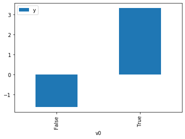
# data['df'] is just a regular pandas.DataFrame
df.causal.do(x=treatment,
                     variable_types={treatment: 'b', outcome: 'c', common_cause: 'c'},
                     outcome=outcome,
                     common_causes=[common_cause]).groupby(treatment).mean().plot(y=outcome, kind='bar')
WARNING:dowhy.causal_model:Causal Graph not provided. DoWhy will construct a graph based on data inputs.
INFO:dowhy.causal_graph:If this is observed data (not from a randomized experiment), there might always be missing confounders. Adding a node named "Unobserved Confounders" to reflect this.
INFO:dowhy.causal_model:Model to find the causal effect of treatment ['v0'] on outcome ['y']
INFO:dowhy.causal_identifier:Common causes of treatment and outcome:['W0', 'U']
WARNING:dowhy.causal_identifier:If this is observed data (not from a randomized experiment), there might always be missing confounders. Causal effect cannot be identified perfectly.
WARN: Do you want to continue by ignoring any unobserved confounders? (use proceed_when_unidentifiable=True to disable this prompt) [y/n] y
INFO:dowhy.causal_identifier:Instrumental variables for treatment and outcome:[]
INFO:dowhy.do_sampler:Using WeightingSampler for do sampling.
INFO:dowhy.do_sampler:Caution: do samplers assume iid data.
[4]:
<matplotlib.axes._subplots.AxesSubplot at 0x7f0f4a609e80>
[5]:
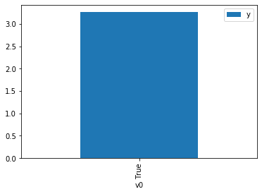
df.causal.do(x={treatment: 1},
              variable_types={treatment:'b', outcome: 'c', common_cause: 'c'},
              outcome=outcome,
              method='weighting',
              common_causes=[common_cause],
              proceed_when_unidentifiable=True).groupby(treatment).mean().plot(y=outcome, kind='bar')
WARNING:dowhy.causal_model:Causal Graph not provided. DoWhy will construct a graph based on data inputs.
INFO:dowhy.causal_graph:If this is observed data (not from a randomized experiment), there might always be missing confounders. Adding a node named "Unobserved Confounders" to reflect this.
INFO:dowhy.causal_model:Model to find the causal effect of treatment ['v0'] on outcome ['y']
INFO:dowhy.causal_identifier:Common causes of treatment and outcome:['W0', 'U']
WARNING:dowhy.causal_identifier:If this is observed data (not from a randomized experiment), there might always be missing confounders. Causal effect cannot be identified perfectly.
INFO:dowhy.causal_identifier:Continuing by ignoring these unobserved confounders because proceed_when_unidentifiable flag is True.
INFO:dowhy.causal_identifier:Instrumental variables for treatment and outcome:[]
INFO:dowhy.do_sampler:Using WeightingSampler for do sampling.
INFO:dowhy.do_sampler:Caution: do samplers assume iid data.
[5]:
<matplotlib.axes._subplots.AxesSubplot at 0x7f0f48316358>
[6]:
cdf_1 = df.causal.do(x={treatment: 1},
              variable_types={treatment: 'b', outcome: 'c', common_cause: 'c'},
              outcome=outcome,
              dot_graph=data['dot_graph'],
              proceed_when_unidentifiable=True)

cdf_0 = df.causal.do(x={treatment: 0},
              variable_types={treatment: 'b', outcome: 'c', common_cause: 'c'},
              outcome=outcome,
              dot_graph=data['dot_graph'],
              proceed_when_unidentifiable=True)
INFO:dowhy.causal_model:Model to find the causal effect of treatment ['v0'] on outcome ['y']
INFO:dowhy.causal_identifier:Common causes of treatment and outcome:['W0', 'U']
WARNING:dowhy.causal_identifier:If this is observed data (not from a randomized experiment), there might always be missing confounders. Causal effect cannot be identified perfectly.
INFO:dowhy.causal_identifier:Continuing by ignoring these unobserved confounders because proceed_when_unidentifiable flag is True.
INFO:dowhy.causal_identifier:Instrumental variables for treatment and outcome:[]
INFO:dowhy.do_sampler:Using WeightingSampler for do sampling.
INFO:dowhy.do_sampler:Caution: do samplers assume iid data.
[7]:
cdf_0
[7]:
| W0 | v0 | y | propensity_score | weight | |
|---|---|---|---|---|---|
| 0 | -0.583286 | False | -2.456860 | 0.574597 | 1.740350 |
| 1 | -1.853274 | False | -3.699267 | 0.754520 | 1.325346 |
| 2 | -1.530711 | False | -4.384006 | 0.713824 | 1.400906 |
| 3 | -0.036469 | False | -2.269524 | 0.486654 | 2.054847 |
| 4 | -1.749115 | False | -3.311137 | 0.741816 | 1.348043 |
| ... | ... | ... | ... | ... | ... |
| 995 | -1.227516 | False | -0.875867 | 0.672107 | 1.487859 |
| 996 | -0.405553 | False | -1.427872 | 0.546258 | 1.830637 |
| 997 | 0.230046 | False | 0.328777 | 0.443752 | 2.253509 |
| 998 | -2.157752 | False | -4.830362 | 0.789181 | 1.267136 |
| 999 | -0.453149 | False | -2.167928 | 0.553884 | 1.805431 |
1000 rows × 5 columns
[8]:
cdf_1
[8]:
| W0 | v0 | y | propensity_score | weight | |
|---|---|---|---|---|---|
| 0 | -0.229733 | True | 4.754793 | 0.482075 | 2.074366 |
| 1 | -0.238390 | True | 4.487643 | 0.480676 | 2.080404 |
| 2 | -2.161507 | True | -1.700668 | 0.210415 | 4.752520 |
| 3 | -1.639879 | True | 2.173829 | 0.271959 | 3.677028 |
| 4 | 0.030840 | True | 4.465655 | 0.524224 | 1.907580 |
| ... | ... | ... | ... | ... | ... |
| 995 | -1.688769 | True | 2.404017 | 0.265737 | 3.763121 |
| 996 | -0.910527 | True | 2.528176 | 0.374608 | 2.669460 |
| 997 | -2.838431 | True | -0.226373 | 0.146704 | 6.816457 |
| 998 | 0.429132 | True | 6.865883 | 0.587791 | 1.701285 |
| 999 | -1.509348 | True | 2.153207 | 0.289010 | 3.460088 |
1000 rows × 5 columns
Comparing the estimate to Linear Regression
First, estimating the effect using the causal data frame, and the 95% confidence interval.
[9]:
(cdf_1['y'] - cdf_0['y']).mean()
[9]:
$\displaystyle 5.006194579687894$
[10]:
1.96*(cdf_1['y'] - cdf_0['y']).std() / np.sqrt(len(df))
[10]:
$\displaystyle 0.2245958282589085$
Comparing to the estimate from OLS.
[11]:
model = OLS(np.asarray(df[outcome]), np.asarray(df[[common_cause, treatment]], dtype=np.float64))
result = model.fit()
result.summary()
[11]:
| Dep. Variable: | y | R-squared (uncentered): | 0.938 |
|---|---|---|---|
| Model: | OLS | Adj. R-squared (uncentered): | 0.938 |
| Method: | Least Squares | F-statistic: | 7544. |
| Date: | Tue, 07 Jan 2020 | Prob (F-statistic): | 0.00 |
| Time: | 11:54:35 | Log-Likelihood: | -1408.7 |
| No. Observations: | 1000 | AIC: | 2821. |
| Df Residuals: | 998 | BIC: | 2831. |
| Df Model: | 2 | ||
| Covariance Type: | nonrobust |
| coef | std err | t | P>|t| | [0.025 | 0.975] | |
|---|---|---|---|---|---|---|
| x1 | 2.2679 | 0.025 | 89.049 | 0.000 | 2.218 | 2.318 |
| x2 | 5.0091 | 0.050 | 100.297 | 0.000 | 4.911 | 5.107 |
| Omnibus: | 2.664 | Durbin-Watson: | 2.034 |
|---|---|---|---|
| Prob(Omnibus): | 0.264 | Jarque-Bera (JB): | 2.431 |
| Skew: | -0.049 | Prob(JB): | 0.297 |
| Kurtosis: | 2.779 | Cond. No. | 2.03 |
Warnings:
[1] Standard Errors assume that the covariance matrix of the errors is correctly specified.