Modeling Graphical Causal Models (GCMs)#
To perform causal tasks based on graphical causal models, such as root cause analysis or quantifying the causal strength of edges, we also have to know the nature of underlying data-generating process of variables. A causal graph by itself, being a diagram, does not have any information about the data-generating process.
All main features of the GCM-based inference in DoWhy are built around the concept of graphical causal models. A graphical causal model consists of a causal direct acyclic graph (DAG) of variables and a causal mechanism for each of the variables. A causal mechanism defines the conditional distribution of a variable given its parents in the graph, or, in case of root node variables, simply its distribution. This is, for non-root nodes, we model a node \(X_i\) as \(X_i = f(PA_{X_i}, N_i)\), where \(PA_{X_i}\) are the parents of \(X_i\) and \(N_i\) is unobserved noise that is assumed to be independent of \(PA_{X_i}\) (causal sufficiency).
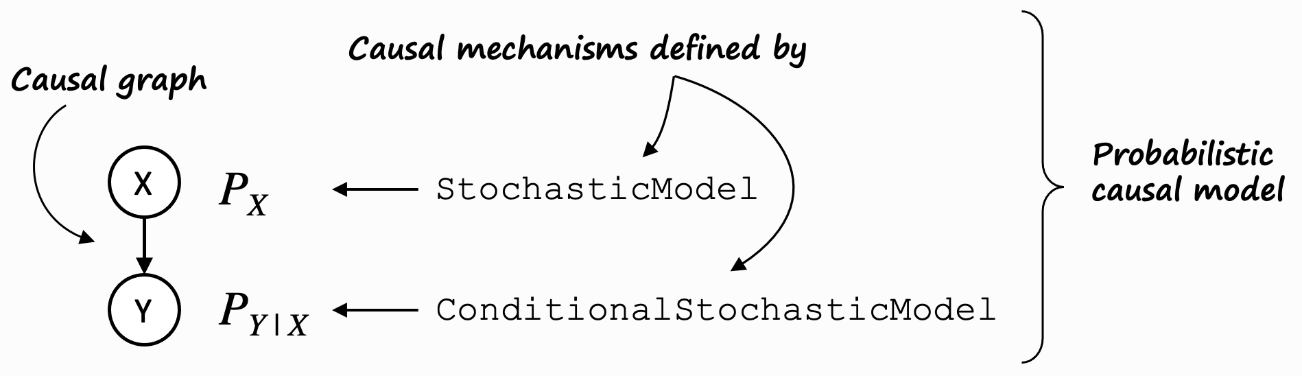
The most general case of a GCM is a probabilistic causal model (PCM), where causal mechanisms are defined by
conditional stochastic models and stochastic models. In the dowhy.gcm package, these are represented by
ProbabilisticCausalModel, ConditionalStochasticModel, and StochasticModel.
In practical terms however, we often use invertible structural causal models (SCMs) to represent our GCMs, and the causal mechanisms are defined by functional causal models (FCMs) for non-root nodes and stochastic models for root nodes. An invertible SCM implements the same traits as a PCM, but on top of that, its FCMs allow us to reason further about its data generation process based on parents and noise, and hence, allow us e.g. to compute counterfactuals. See section Types of graphical causal models for more details about the type of graphs and their implications.
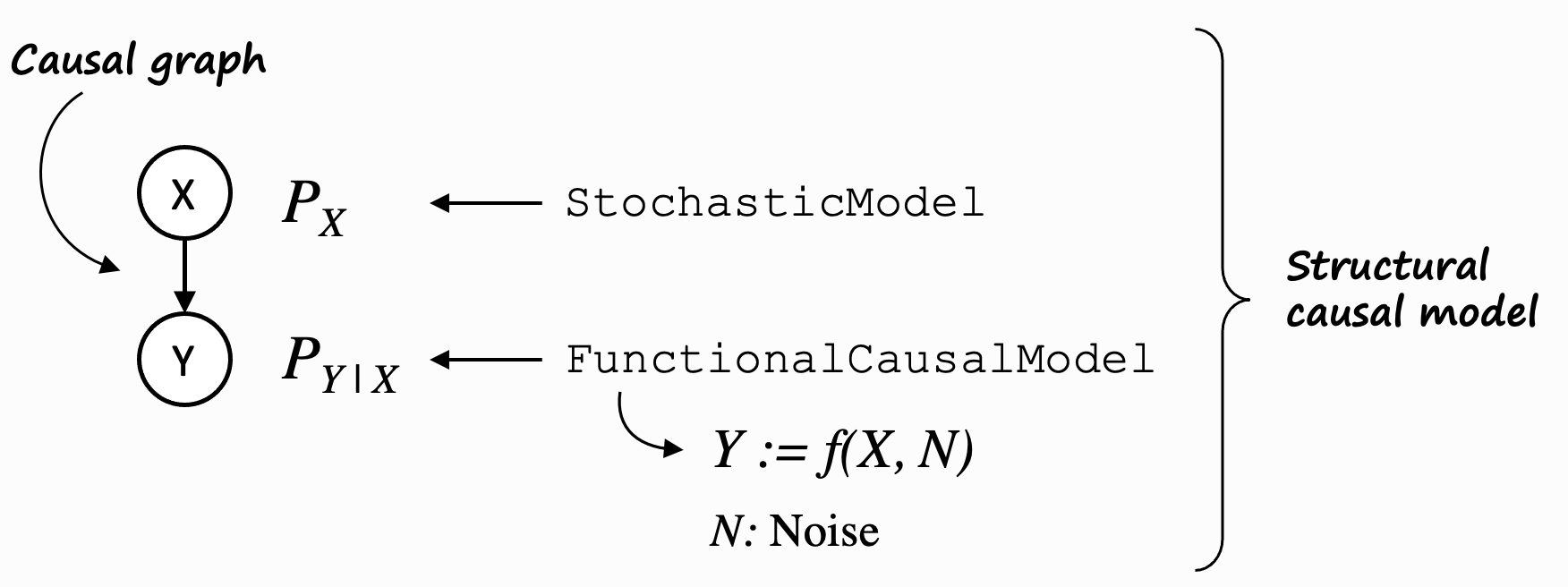
To keep this introduction simple, we will stick with SCMs for now.
As mentioned above, a causal mechanism describes how the values of a node are influenced by the values of its parent nodes. We will dive much deeper into the details of causal mechanisms and their meaning in section Customizing Causal Mechanism Assignment. But for this introduction, we will treat them as an opaque thing that is needed to answer causal questions.
To introduce this data-generating process, we use an SCM that’s built on top of our causal graph:
>>> from dowhy import gcm
>>> import networkx as nx
>>> causal_model = gcm.StructuralCausalModel(nx.DiGraph([("X", "Y"), ("Y", "Z")]))
At this point we would normally load our dataset. For this introduction, we generate some synthetic data instead. The API takes data in form of Pandas DataFrames:
>>> import numpy as np, pandas as pd
>>> X = np.random.normal(loc=0, scale=1, size=1000)
>>> Y = 2 * X + np.random.normal(loc=0, scale=1, size=1000)
>>> Z = 3 * Y + np.random.normal(loc=0, scale=1, size=1000)
>>> data = pd.DataFrame(data=dict(X=X, Y=Y, Z=Z))
>>> data.head()
          X         Y          Z
0 -2.253500 -3.638579 -10.370047
1 -1.078337 -2.114581  -6.028030
2 -0.962719 -2.157896  -5.750563
3 -0.300316 -0.440721  -2.619954
4  0.127419  0.158185   1.555927
Note how the columns X, Y, Z correspond to our nodes X, Y, Z in the graph constructed above. We can also see how the values of X influence the values of Y and how the values of Y influence the values of Z in that data set.
The causal model created above allows us now to assign causal mechanisms to each node in the form of functional causal
models. Here, these mechanism can either be assigned manually if, for instance, prior knowledge about certain causal
relationships are known or they can be assigned automatically using the auto module. For the latter,
we simply call:
>>> gcm.auto.assign_causal_mechanisms(causal_model, data)
In case we want to have more control over the assigned mechanisms, we can do this manually as well. For instance, we can can assign an empirical distribution to the root node X and linear additive noise models to nodes Y and Z:
>>> causal_model.set_causal_mechanism('X', gcm.EmpiricalDistribution())
>>> causal_model.set_causal_mechanism('Y', gcm.AdditiveNoiseModel(gcm.ml.create_linear_regressor()))
>>> causal_model.set_causal_mechanism('Z', gcm.AdditiveNoiseModel(gcm.ml.create_linear_regressor()))
Section Customizing Causal Mechanism Assignment will go into more detail on how one can even define a completely customized model or add their own implementation.
In the real world, the data comes as an opaque stream of values, where we typically don’t know how one variable influences another. The graphical causal models can help us to deconstruct these causal relationships again, even though we didn’t know them before.
Fitting an SCM to the data#
With the data at hand and the graph constructed earlier, we can now train the SCM using fit:
>>> gcm.fit(causal_model, data)
Fitting means, we learn the generative models of the variables in the SCM according to the data.
The causal model is now ready to be used for Performing Causal Tasks.
Evaluating a fitted SCM#
For evaluating the fitted model, see Evaluate a GCM.