Evaluate a GCM#
Modeling a graphical causal model (GCM) requires various assumptions and choices of models, all of which can influence the performance and accuracy of the model. Some examples of the required assumptions include:
Graph Structure: Correctly specifying the causal directions between variables is crucial. For example, it is logical to say that rain causes the street to be wet, whereas asserting that a wet street causes rain does not make sense. If these relationships are modeled incorrectly, the resultant causal statements will be misleading. However, it is important to note that while this example is quite straightforward, models typically exhibit some level of robustness to misspecifications. Particularly, the impact of misspecification tends to be less severe in larger graphs. Additionally, the severity of misspecifications can vary; for instance, defining an incorrect causal direction is generally more problematic than including too many (upstream) nodes as potential parents of a node.
Since a causal graph structure defines assumptions about the (conditional) independencies between variables, one can falsify a given graph structure. For instance, in a chain X→Y→Z, we know that X and Z have to be independent given Y. If this is not the case, we have some evidence that the given graph is wrong. However, on the other hand, without stronger assumptions, we cannot confirm the correctness of a graph. Following the chain example, if we flip both edges, the conditional independence statement (X independent of Z given Y) would still hold.
Causal Mechanism Assumption: To model the causal data generation process, we represent each node with a causal mechanism of the form \(X_i = f_i(PA_i, N_i)\), where \(N_i\) denotes unobserved noise, and \(PA_i\) represents the causal parents of \(X_i\). In this context, we require an additional assumption regarding the form of the function \(f_i\). For continuous variables, for instance, it is common to model \(f_i\) using an additive noise model of the form \(X_i = f_i(PA_i) + N_i\). However, this representation may not be accurate if the true relationship is different (e.g., multiplicative). Thus, the type of causal mechanism is another factor that can influence the results. Generally, however, the additive noise model assumption in the continuous case tends to be relatively robust to violations in practice.
Model Selection: The previous two points focused solely on accurately representing the causal relationships between variables. Now, the process of model selection adds an additional layer. Sticking to the additive noise model \(X_i = f_i(PA_i) + N_i\) as an example, the challenge in model selection lies in determining the optimal model for \(f_i\). Ideally, this would be the model that minimizes the mean squared error.
Given the multitude of factors that impact the performance of a GCM, each with their own metrics and challenges,
dowhy.gcm has a module that aims at evaluating a fitted GCM and providing an overview of different evaluation
metrics. Furthermore, if the auto assignment is used, we can obtain an overview of the evaluated models and
performances in the selection process.
Summary of auto assignment#
If prior knowledge about causal relationships is available, it is always recommended to use that knowledge to model the causal mechanisms accordingly. However, if one does not have enough insights, the auto assignment function for GCMs can help automatically select an appropriate causal mechanism for each node based on the given data. The auto assignment does two things: 1) Select an appropriate causal mechanism and 2) select the best performing model from a small model zoo.
When using the auto assignment function, we can obtain additional insights into the model selection process, such as the types of causal mechanisms considered and the evaluated models with their performances. To illustrate this, consider the chain structure example X→Y→Z again:
>>> import numpy as np, pandas as pd
>>> import networkx as nx
>>> import dowhy.gcm as gcm
>>>
>>> X = np.random.normal(loc=0, scale=1, size=1000)
>>> Y = 2 * X + np.random.normal(loc=0, scale=1, size=1000)
>>> Z = 3 * Y + np.random.normal(loc=0, scale=1, size=1000)
>>> data = pd.DataFrame(data=dict(X=X, Y=Y, Z=Z))
>>>
>>> causal_model = gcm.StructuralCausalModel(nx.DiGraph([('X', 'Y'), ('Y', 'Z')]))
>>> summary_auto_assignment = gcm.auto.assign_causal_mechanisms(causal_model, data)
>>> print(summary_auto_assignment)
When using this auto assignment function, the given data is used to automatically assign a causal mechanism to each node. Note that causal mechanisms can also be customized and assigned manually.
The following types of causal mechanisms are considered for the automatic selection:

If root node:
An empirical distribution, i.e., the distribution is represented by randomly sampling from the provided data. This provides a flexible and non-parametric way to model the marginal distribution and is valid for all types of data modalities.

If non-root node and the data is continuous:
Additive Noise Models (ANM) of the form X_i = f(PA_i) + N_i, where PA_i are the parents of X_i and the unobserved noise N_i is assumed to be independent of PA_i.To select the best model for f, different regression models are evaluated and the model with the smallest mean squared error is selected.Note that minimizing the mean squared error here is equivalent to selecting the best choice of an ANM.

If non-root node and the data is discrete:
Discrete Additive Noise Models have almost the same definition as non-discrete ANMs, but come with an additional constraint for f to only return discrete values.
Note that 'discrete' here refers to numerical values with an order. If the data is categorical, consider representing them as strings to ensure proper model selection.

If non-root node and the data is categorical:
A functional causal model based on a classifier, i.e., X_i = f(PA_i, N_i).
Here, N_i follows a uniform distribution on [0, 1] and is used to randomly sample a class (category) using the conditional probability distribution produced by a classification model. Here, different model classes are evaluated using the log loss metric and the best performing model class is selected.

In total, 3 nodes were analyzed:

--- Node: X
Node X is a root node. Therefore, assigning 'Empirical Distribution' to the node representing the marginal distribution.

--- Node: Y
Node Y is a non-root node with continuous data. Assigning 'AdditiveNoiseModel using LinearRegression' to the node.
This represents the causal relationship as Y := f(X) + N.
For the model selection, the following models were evaluated on the mean squared error (MSE) metric:
LinearRegression: 0.9978767184153945
Pipeline(steps=[('polynomialfeatures', PolynomialFeatures(include_bias=False)),
                ('linearregression', LinearRegression)]): 1.00448207264867
HistGradientBoostingRegressor: 1.1386270868995179

--- Node: Z
Node Z is a non-root node with continuous data. Assigning 'AdditiveNoiseModel using LinearRegression' to the node.
This represents the causal relationship as Z := f(Y) + N.
For the model selection, the following models were evaluated on the mean squared error (MSE) metric:
LinearRegression: 1.0240822102491627
Pipeline(steps=[('polynomialfeatures', PolynomialFeatures(include_bias=False)),
                ('linearregression', LinearRegression)]): 1.02567150836141
HistGradientBoostingRegressor: 1.358002751994007

===Note===
Note, based on the selected auto assignment quality, the set of evaluated models changes.
For more insights toward the quality of the fitted graphical causal model, consider using the evaluate_causal_model function after fitting the causal mechanisms.
In this scenario, an empirical distribution is assigned to the root node X, while additive noise models are used for nodes Y and Z (see Types of graphical causal models for more details about the causal mechanism types). In both of these cases, a linear regression model demonstrated the best performance in terms of minimizing the mean squared error. A list of evaluated models and their performance is also available. Since we used the default parameter for the auto assignment, only a small model zoo is evaluated. However, we can also adjust the assigment quality to extend it to more models.
After assigning causal mechanisms to each node, the subsequent step involves fitting these mechanisms to the data:
>>> gcm.fit(causal_model, data)
Evaluating a fitted GCM#
The causal model has been fitted and can be used for different causal questions. However, we might be interested in obtaining some insights into the causal model performance first, i.e., we might wonder:
How well do my causal mechanisms perform?
Is the additive noise model assumption even valid for my data?
Does the GCM capture the joint distribution of the observed data?
Is my causal graph structure compatible with the data?
For this, we can use the causal model evaluation function, which provides us with some insights into the overall model performance and whether our assumptions hold:
>>> summary_evaluation = gcm.evaluate_causal_model(causal_model, data, compare_mechanism_baselines=True)
>>> print(summary_evaluation)
Evaluated the performance of the causal mechanisms and the invertibility assumption of the causal mechanisms and the overall average KL divergence between generated and observed distribution and the graph structure. The results are as follows:
==== Evaluation of Causal Mechanisms ====
The used evaluation metrics are:
- KL divergence (only for root-nodes): Evaluates the divergence between the generated and the observed distribution.
- Mean Squared Error (MSE): Evaluates the average squared differences between the observed values and the conditional expectation of the causal mechanisms.
- Normalized MSE (NMSE): The MSE normalized by the standard deviation for better comparison.
- R2 coefficient: Indicates how much variance is explained by the conditional expectations of the mechanisms. Note, however, that this can be misleading for nonlinear relationships.
- F1 score (only for categorical non-root nodes): The harmonic mean of the precision and recall indicating the goodness of the underlying classifier model.
- (normalized) Continuous Ranked Probability Score (CRPS): The CRPS generalizes the Mean Absolute Percentage Error to probabilistic predictions. This gives insights into the accuracy and calibration of the causal mechanisms.
NOTE: Every metric focuses on different aspects and they might not consistently indicate a good or bad performance.
We will mostly utilize the CRPS for comparing and interpreting the performance of the mechanisms, since this captures the most important properties for the causal model.
--- Node X
- The KL divergence between generated and observed distribution is 0.04082997872632467.
The estimated KL divergence indicates an overall very good representation of the data distribution.
--- Node Y
- The MSE is 0.9295878353315775.
- The NMSE is 0.44191515264388137.
- The R2 coefficient is 0.8038281270395207.
- The normalized CRPS is 0.25235753447337383.
The estimated CRPS indicates a good model performance.
The mechanism is better or equally good than all 7 baseline mechanisms.
--- Node Z
- The MSE is 0.9485970223031653.
- The NMSE is 0.14749131486369138.
- The R2 coefficient is 0.9781306148527433.
- The normalized CRPS is 0.08386782069483441.
The estimated CRPS indicates a very good model performance.
The mechanism is better or equally good than all 7 baseline mechanisms.
==== Evaluation of Invertible Functional Causal Model Assumption ====
--- The model assumption for node Y is not rejected with a p-value of 1.0 (after potential adjustment) and a significance level of 0.05.
This implies that the model assumption might be valid.
--- The model assumption for node Z is not rejected with a p-value of 1.0 (after potential adjustment) and a significance level of 0.05.
This implies that the model assumption might be valid.
Note that these results are based on statistical independence tests, and the fact that the assumption was not rejected does not necessarily imply that it is correct. There is just no evidence against it.
==== Evaluation of Generated Distribution ====
The overall average KL divergence between the generated and observed distribution is 0.015438550831663324
The estimated KL divergence indicates an overall very good representation of the data distribution.
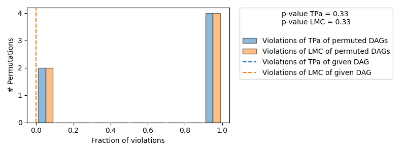
==== Evaluation of the Causal Graph Structure ====
+-------------------------------------------------------------------------------------------------------+
| Falsification Summary |
+-------------------------------------------------------------------------------------------------------+
| The given DAG is not informative because 2 / 6 of the permutations lie in the Markov |
| equivalence class of the given DAG (p-value: 0.33). |
| The given DAG violates 0/1 LMCs and is better than 66.7% of the permuted DAGs (p-value: 0.33). |
| Based on the provided significance level (0.2) and because the DAG is not informative, |
| we do not reject the DAG. |
+-------------------------------------------------------------------------------------------------------+
==== NOTE ====
Always double check the made model assumptions with respect to the graph structure and choice of causal mechanisms.
All these evaluations give some insight into the goodness of the causal model, but should not be overinterpreted, since some causal relationships can be intrinsically hard to model. Furthermore, many algorithms are fairly robust against misspecifications or poor performances of causal mechanisms.
As we see, we get a detailed overview of different evaluations:
Evaluation of Causal Mechanisms: Evaluation of the causal mechanisms with respect to their model performance. For non-root nodes, the most important measure is the (normalized) Continuous Ranked Probability Score (CRPS), which provides insights into the mechanism’s accuracy and its calibration as a probabilistic model. It further lists other metrics such as the mean squared error (MSE), the MSE normalized by the variance (denoted as NMSE), the R2 coefficient and, in the case of categorical variables, the F1 score. If the node is a root node, the KL divergence between the generated and observed data distributions is measured.
Optionally, we can set the compare_mechanism_baselines parameter to True in order
to compare the mechanisms with some baseline models. This gives us better insights into how the mechanisms perform in
comparison to other models. Note, however, that this can take significant time for larger graphs.
Evaluation of Invertible Functional Causal Model Assumption: If the causal mechanism is an invertible functional causal model, we can validate if the assumption holds true. Note that an invertible function here means with respect to the noise, i.e., an additive noise model \(X_i = f_i(PA_i) + N_i\) and, more generally, post non-linear models \(X_i = g_i(f_i(PA_i) + N_i)\) where \(g_i\) is invertible are examples for such types of mechanisms. In this case, the estimated noise based on the observation should be independent of the inputs.
Evaluation of Generated Distribution: Since the GCM is able to generate new samples from the learned distributions, we can evaluate whether the generated (joint) distribution coincides with the observed one. Here, the difference should be as small as possible. To make the KL divergence estimation practical for potentially large graphs, this is approximated by taking the mean over the KL divergence between the generated and observed marginal distributions for each node.
Evaluation of the Causal Graph Structure: As discussed above, the graph structure should represent the (conditional) independencies in the observed data (assuming faithfulness). This can be exploited to obtain some insights on whether the given graph violates the (in)dependence structures based on the data by running different independence tests. For this, an algorithm is used that checks whether the graph can be rejected and whether one is even able to obtain an informative insight from such independence tests.
Note that all these evaluation methods only provide some insights into the provided GCM, but cannot fully confirm the correctness of a learned model. More details about the metrics and evaluation methods, please see the corresponding docstring of the method.