Anomaly Attribution#
When we observe an anomaly in a target node of interest, we can address the question:
How much did each of the upstream nodes and the target node contribute to the observed anomaly?
Through this, we identify and specifically quantify the contribution of each node to the anomalous observation. This method is based on the paper:
Kailash Budhathoki, Lenon Minorics, Patrick Blöbaum, Dominik Janzing. Causal structure-based root cause analysis of outliers International Conference on Machine Learning, 2022
How to use it#
First, let’s generate some example data of a simple chain X → Y → Z → W:
>>> import numpy as np, pandas as pd, networkx as nx
>>> from dowhy import gcm
>>> X = np.random.uniform(low=-5, high=5, size=1000)
>>> Y = 0.5 * X + np.random.normal(loc=0, scale=1, size=1000)
>>> Z = 2 * Y + np.random.normal(loc=0, scale=1, size=1000)
>>> W = 3 * Z + np.random.normal(loc=0, scale=1, size=1000)
>>> data = pd.DataFrame(data=dict(X=X, Y=Y, Z=Z, W=W))
Next, we model cause-effect relationships as an invertible structural causal model and fit it to the data. We use the auto module to assign causal mechanisms automatically:
>>> causal_model = gcm.InvertibleStructuralCausalModel(nx.DiGraph([('X', 'Y'), ('Y', 'Z'), ('Z', 'W')]))  # X -> Y -> Z -> W
>>> gcm.auto.assign_causal_mechanisms(causal_model, data)
>>> gcm.fit(causal_model, data)
Then, we create an anomaly. For instance, we set the noise of \(Y\) to an unusually high value:
>>> X = np.random.uniform(low=-5, high=5)  # Sample from its normal distribution.
>>> Y = 0.5 * X + 5  # Here, we set the noise of Y to 5, which is unusually high.
>>> Z = 2 * Y
>>> W = 3 * Z
>>> anomalous_data = pd.DataFrame(data=dict(X=[X], Y=[Y], Z=[Z], W=[W]))  # This data frame consist of only one sample here.
Here, \(Y\) is the root cause, which leads to \(Y, Z\) and \(W\) being anomalous. We can now get the anomaly attribution scores of our target node of interest (e.g., \(W\)).
>>> attribution_scores = gcm.attribute_anomalies(causal_model, 'W', anomaly_samples=anomalous_data)
>>> attribution_scores
    {'X': array([0.59766433]), 'Y': array([7.40955119]), 'Z': array([-0.00236857]), 'W': array([0.0018539])}
Although we use a linear relationship here, the method can also accommodate arbitrary non-linear relationships. There could also be multiple root causes.
Interpretation of results: We estimated the contribution of the ancestors of \(W\), including \(W\) itself, to the observed anomaly. While all nodes contribute to some extent, \(Y\) is the standout. Note that \(Z\) is also anomalous due to \(Y\), but it merely inherits the high value from \(Y\). The attribution method is able identify this and distinguishes between the contributions of \(Y\) and \(Z\). In case of a negative contribution, the corresponding node even decreases the likelihood of an anomaly, i.e., reducing its apparent severity.
For a detailed interpretation of the score, see the referenced paper. The following section also offers some intuition.
Understanding the method#
In this method, we use invertible causal mechanisms to reconstruct and modify the noise leading to a certain observation. We then ask, “If the noise value of a specific node was from its ‘normal’ distribution, would we still have observed an anomalous value in the target node?”. The change in the severity of the anomaly in the target node after altering an upstream noise variable’s value, based on its learned distribution, indicates the node’s contribution to the anomaly. The advantage of using the noise value over the actual node value is that we measure only the influence originating from the node and not inherited from its parents.
The process can be summarized as:
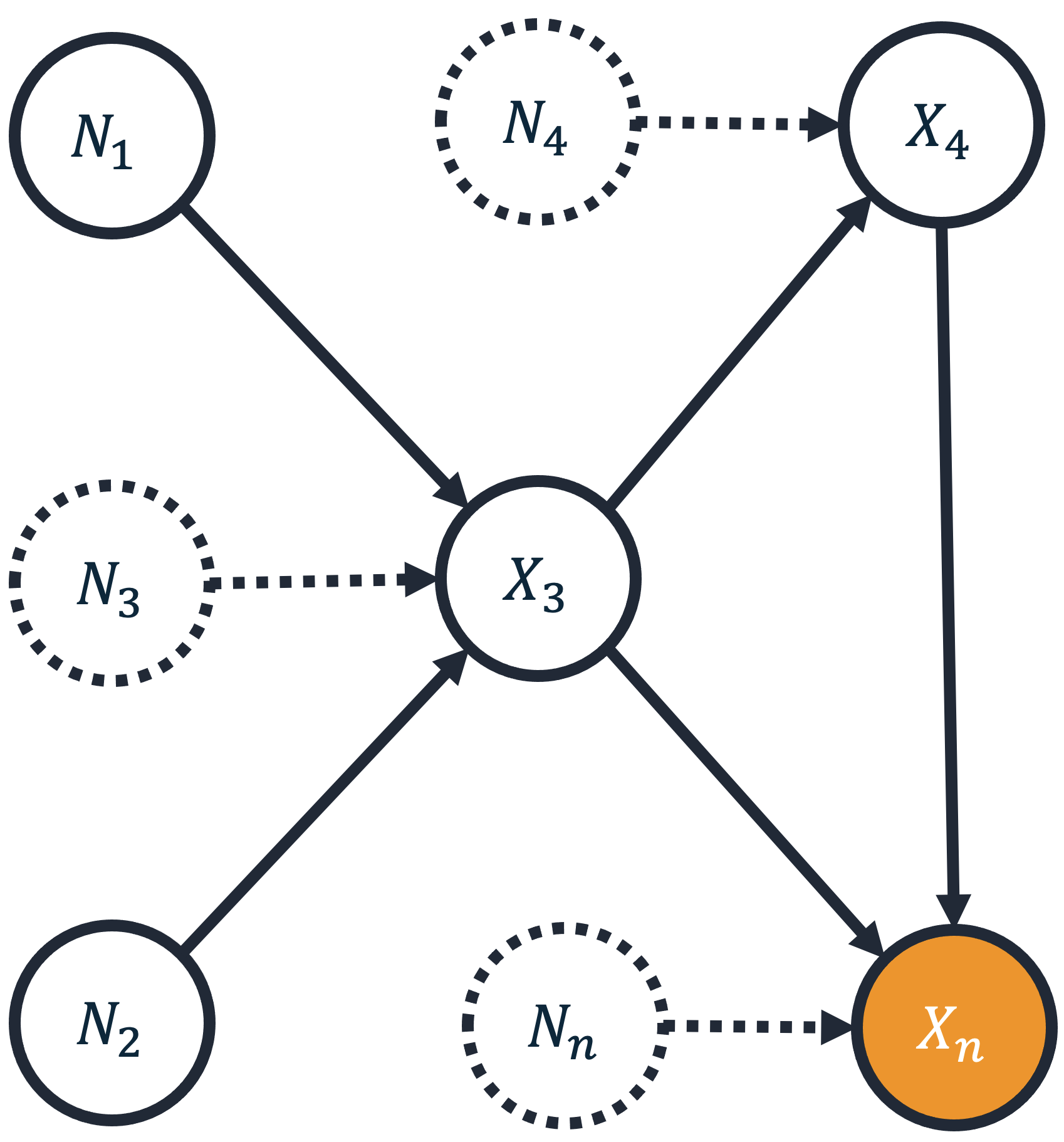
Define an outlier score for target variable \(X_n\) as \(S(x_n) := -log P(g(X_n) \geq g(x_n))\) for some feature map \(g\). Here, \(g\) is an arbitrary anomaly scorer, such as an isolation forest, median/mean difference, or any other model giving an anomaly score. The information theoretic score \(S(x_n)\) for an observation \(x_n\) is then scale invariant and independent of the choice of anomaly scorer.
Define the contribution of node \(j\) by \(log \frac{P(g(X_n) \geq g(x_n) | \text{replace all noise values } n_1, ..., n_{j-1} \text{ with random values})}{P(g(X_n) \geq g(x_n) | \text{replace all noise values } n_1, ..., n_j \text{ with random values})}\), where ‘random values’ are relative to the learned noise distribution. This log-ratio measures how randomizing noise \(N_j\) reduces the likelihood of the outlier event.
Symmetrize the contribution across all orderings to eliminate ambiguity from node reordering. We use a Shapley symmetrization for this.
The final Shapley values sum up to the outlier score \(S(x_n)\).
This approach’s crucial property is that only rare events can get high contributions; common events can’t explain rare ones.
Simple Example: A basic and straightforward example where we can directly obtain the contributions is when we have two dice, one with four sides and another with 100 sides (e.g., from a D&D game). If we roll the dice and get (1, 1), the ‘outlier’ score for this event is \(log(4 \cdot 100) = log(4) + log(100)\). Here, the contributions of each die to this event are directly based on the sum; the four-sided die contributed 23%, and the 100-sided die contributed 77% to the (1, 1) event.