Lalonde Pandas API Example
by Adam Kelleher
We’ll run through a quick example using the high-level Python API for the DoSampler. The DoSampler is different from most classic causal effect estimators. Instead of estimating statistics under interventions, it aims to provide the generality of Pearlian causal inference. In that context, the joint distribution of the variables under an intervention is the quantity of interest. It’s hard to represent a joint distribution nonparametrically, so instead we provide a sample from that distribution, which we call a “do” sample.
Here, when you specify an outcome, that is the variable you’re sampling under an intervention. We still have to do the usual process of making sure the quantity (the conditional interventional distribution of the outcome) is identifiable. We leverage the familiar components of the rest of the package to do that “under the hood”. You’ll notice some similarity in the kwargs for the DoSampler.
[1]:
import os, sys
sys.path.append(os.path.abspath("../../../"))
Getting the Data
First, download the data from the LaLonde example.
[2]:
import dowhy.datasets

lalonde = dowhy.datasets.lalonde_dataset()
The causal Namespace
We’ve created a “namespace” for pandas.DataFrames containing causal inference methods. You can access it here with lalonde.causal, where lalonde is our pandas.DataFrame, and causal contains all our new methods! These methods are magically loaded into your existing (and future) dataframes when you import dowhy.api.
[3]:
import dowhy.api
Now that we have the causal namespace, lets give it a try!
The do Operation
The key feature here is the do method, which produces a new dataframe replacing the treatment variable with values specified, and the outcome with a sample from the interventional distribution of the outcome. If you don’t specify a value for the treatment, it leaves the treatment untouched:
[4]:
do_df = lalonde.causal.do(x='treat',
                          outcome='re78',
                          common_causes=['nodegr', 'black', 'hisp', 'age', 'educ', 'married'],
                          variable_types={'age': 'c', 'educ':'c', 'black': 'd', 'hisp': 'd',
                                          'married': 'd', 'nodegr': 'd','re78': 'c', 'treat': 'b'},
                         proceed_when_unidentifiable=True)
Notice you get the usual output and prompts about identifiability. This is all dowhy under the hood!
We now have an interventional sample in do_df. It looks very similar to the original dataframe. Compare them:
[5]:
lalonde.head()
[5]:
| treat | age | educ | black | hisp | married | nodegr | re74 | re75 | re78 | u74 | u75 | |
|---|---|---|---|---|---|---|---|---|---|---|---|---|
| 0 | False | 23.0 | 10.0 | 1.0 | 0.0 | 0.0 | 1.0 | 0.0 | 0.0 | 0.00 | 1.0 | 1.0 |
| 1 | False | 26.0 | 12.0 | 0.0 | 0.0 | 0.0 | 0.0 | 0.0 | 0.0 | 12383.68 | 1.0 | 1.0 |
| 2 | False | 22.0 | 9.0 | 1.0 | 0.0 | 0.0 | 1.0 | 0.0 | 0.0 | 0.00 | 1.0 | 1.0 |
| 3 | False | 18.0 | 9.0 | 1.0 | 0.0 | 0.0 | 1.0 | 0.0 | 0.0 | 10740.08 | 1.0 | 1.0 |
| 4 | False | 45.0 | 11.0 | 1.0 | 0.0 | 0.0 | 1.0 | 0.0 | 0.0 | 11796.47 | 1.0 | 1.0 |
[6]:
do_df.head()
[6]:
| treat | age | educ | black | hisp | married | nodegr | re74 | re75 | re78 | u74 | u75 | propensity_score | weight | |
|---|---|---|---|---|---|---|---|---|---|---|---|---|---|---|
| 0 | True | 19.0 | 10.0 | 1.0 | 0.0 | 0.0 | 1.0 | 4121.949 | 6056.754 | 0.000 | 0.0 | 0.0 | 0.364787 | 2.741328 |
| 1 | True | 21.0 | 13.0 | 1.0 | 0.0 | 0.0 | 0.0 | 0.000 | 0.000 | 17094.640 | 1.0 | 1.0 | 0.519464 | 1.925060 |
| 2 | False | 17.0 | 10.0 | 0.0 | 1.0 | 0.0 | 1.0 | 4905.119 | 1168.902 | 11306.270 | 0.0 | 0.0 | 0.741764 | 1.348138 |
| 3 | True | 29.0 | 10.0 | 0.0 | 1.0 | 0.0 | 1.0 | 0.000 | 8853.674 | 5112.014 | 1.0 | 0.0 | 0.273944 | 3.650381 |
| 4 | True | 17.0 | 8.0 | 1.0 | 0.0 | 0.0 | 1.0 | 0.000 | 0.000 | 8061.485 | 1.0 | 1.0 | 0.385366 | 2.594934 |
Treatment Effect Estimation
We could get a naive estimate before for a treatment effect by doing
[7]:
(lalonde[lalonde['treat'] == 1].mean() - lalonde[lalonde['treat'] == 0].mean())['re78']
[7]:
We can do the same with our new sample from the interventional distribution to get a causal effect estimate
[8]:
(do_df[do_df['treat'] == 1].mean() - do_df[do_df['treat'] == 0].mean())['re78']
[8]:
We could get some rough error bars on the outcome using the normal approximation for a 95% confidence interval, like
[9]:
import numpy as np
1.96*np.sqrt((do_df[do_df['treat'] == 1].var()/len(do_df[do_df['treat'] == 1])) +
             (do_df[do_df['treat'] == 0].var()/len(do_df[do_df['treat'] == 0])))['re78']
[9]:
but note that these DO NOT contain propensity score estimation error. For that, a bootstrapping procedure might be more appropriate.
This is just one statistic we can compute from the interventional distribution of 're78'. We can get all of the interventional moments as well, including functions of 're78'. We can leverage the full power of pandas, like
[10]:
do_df['re78'].describe()
[10]:
count      445.000000
mean      5502.694344
std       7368.972876
min          0.000000
25%          0.000000
50%       3343.224000
75%       8551.533000
max      60307.930000
Name: re78, dtype: float64
[11]:
lalonde['re78'].describe()
[11]:
count      445.000000
mean      5300.763699
std       6631.491695
min          0.000000
25%          0.000000
50%       3701.812000
75%       8124.715000
max      60307.930000
Name: re78, dtype: float64
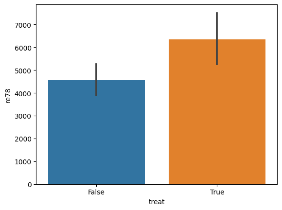
and even plot aggregations, like
[12]:
%matplotlib inline
[13]:
import seaborn as sns

sns.barplot(data=lalonde, x='treat', y='re78')
[13]:
<AxesSubplot: xlabel='treat', ylabel='re78'>
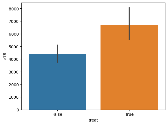
[14]:
sns.barplot(data=do_df, x='treat', y='re78')
[14]:
<AxesSubplot: xlabel='treat', ylabel='re78'>
Specifying Interventions
You can find the distribution of the outcome under an intervention to set the value of the treatment.
[15]:
do_df = lalonde.causal.do(x={'treat': 1},
                          outcome='re78',
                          common_causes=['nodegr', 'black', 'hisp', 'age', 'educ', 'married'],
                          variable_types={'age': 'c', 'educ':'c', 'black': 'd', 'hisp': 'd',
                                          'married': 'd', 'nodegr': 'd','re78': 'c', 'treat': 'b'},
                         proceed_when_unidentifiable=True)
[16]:
do_df.head()
[16]:
| treat | age | educ | black | hisp | married | nodegr | re74 | re75 | re78 | u74 | u75 | propensity_score | weight | |
|---|---|---|---|---|---|---|---|---|---|---|---|---|---|---|
| 0 | True | 27.0 | 10.0 | 1.0 | 0.0 | 1.0 | 1.0 | 0.000 | 0.000 | 18739.930 | 1.0 | 1.0 | 0.427789 | 2.337600 |
| 1 | True | 19.0 | 11.0 | 1.0 | 0.0 | 0.0 | 1.0 | 2305.026 | 2615.276 | 4146.603 | 0.0 | 0.0 | 0.353141 | 2.831729 |
| 2 | True | 27.0 | 10.0 | 1.0 | 0.0 | 1.0 | 1.0 | 0.000 | 0.000 | 18739.930 | 1.0 | 1.0 | 0.427789 | 2.337600 |
| 3 | True | 23.0 | 8.0 | 0.0 | 1.0 | 0.0 | 1.0 | 0.000 | 0.000 | 3881.284 | 1.0 | 1.0 | 0.286242 | 3.493543 |
| 4 | True | 23.0 | 12.0 | 1.0 | 0.0 | 0.0 | 0.0 | 6269.341 | 3039.960 | 8484.239 | 0.0 | 0.0 | 0.535420 | 1.867693 |
This new dataframe gives the distribution of 're78' when 'treat' is set to 1.
For much more detail on how the do method works, check the docstring:
[17]:
help(lalonde.causal.do)
Help on method do in module dowhy.api.causal_data_frame:

do(x, method='weighting', num_cores=1, variable_types={}, outcome=None, params=None, dot_graph=None, common_causes=None, estimand_type='nonparametric-ate', proceed_when_unidentifiable=False, stateful=False) method of dowhy.api.causal_data_frame.CausalAccessor instance
    The do-operation implemented with sampling. This will return a pandas.DataFrame with the outcome
    variable(s) replaced with samples from P(Y|do(X=x)).

    If the value of `x` is left unspecified (e.g. as a string or list), then the original values of `x` are left in
    the DataFrame, and Y is sampled from its respective P(Y|do(x)). If the value of `x` is specified (passed with a
    `dict`, where variable names are keys, and values are specified) then the new `DataFrame` will contain the
    specified values of `x`.

    For some methods, the `variable_types` field must be specified. It should be a `dict`, where the keys are
    variable names, and values are 'o' for ordered discrete, 'u' for un-ordered discrete, 'd' for discrete, or 'c'
    for continuous.

    Inference requires a set of control variables. These can be provided explicitly using `common_causes`, which
    contains a list of variable names to control for. These can be provided implicitly by specifying a causal graph
    with `dot_graph`, from which they will be chosen using the default identification method.

    When the set of control variables can't be identified with the provided assumptions, a prompt will raise to the
    user asking whether to proceed. To automatically over-ride the prompt, you can set the flag
    `proceed_when_unidentifiable` to `True`.

    Some methods build components during inference which are expensive. To retain those components for later
    inference (e.g. successive calls to `do` with different values of `x`), you can set the `stateful` flag to `True`.
    Be cautious about using the `do` operation statefully. State is set on the namespace, rather than the method, so
    can behave unpredictably. To reset the namespace and run statelessly again, you can call the `reset` method.

    :param x: str, list, dict: The causal state on which to intervene, and (optional) its interventional value(s).
    :param method: The inference method to use with the sampler. Currently, `'mcmc'`, `'weighting'`, and
        `'kernel_density'` are supported. The `mcmc` sampler requires `pymc3>=3.7`.
    :param num_cores: int: if the inference method only supports sampling a point at a time, this will parallelize
        sampling.
    :param variable_types: dict: The dictionary containing the variable types. Must contain the union of the causal
        state, control variables, and the outcome.
    :param outcome: str: The outcome variable.
    :param params: dict: extra parameters to set as attributes on the sampler object
    :param dot_graph: str: A string specifying the causal graph.
    :param common_causes: list: A list of strings containing the variable names to control for.
    :param estimand_type: str: 'nonparametric-ate' is the only one currently supported. Others may be added later, to allow for specific, parametric estimands.
    :param proceed_when_unidentifiable: bool: A flag to over-ride user prompts to proceed when effects aren't
        identifiable with the assumptions provided.
    :param stateful: bool: Whether to retain state. By default, the do operation is stateless.

    :return: pandas.DataFrame: A DataFrame containing the sampled outcome