DoWhy: Different estimation methods for causal inference
This is a quick introduction to the DoWhy causal inference library. We will load in a sample dataset and use different methods for estimating the causal effect of a (pre-specified)treatment variable on a (pre-specified) outcome variable.
We will see that not all estimators return the correct effect for this dataset.
First, let us add the required path for Python to find the DoWhy code and load all required packages
[1]:
%load_ext autoreload
%autoreload 2
[2]:
import numpy as np
import pandas as pd
import logging

import dowhy
from dowhy import CausalModel
import dowhy.datasets
Now, let us load a dataset. For simplicity, we simulate a dataset with linear relationships between common causes and treatment, and common causes and outcome.
Beta is the true causal effect.
[3]:
data = dowhy.datasets.linear_dataset(beta=10,
        num_common_causes=5,
        num_instruments = 2,
        num_treatments=1,
        num_samples=10000,
        treatment_is_binary=True,
        outcome_is_binary=False,
        stddev_treatment_noise=10)
df = data["df"]
df
[3]:
| Z0 | Z1 | W0 | W1 | W2 | W3 | W4 | v0 | y | |
|---|---|---|---|---|---|---|---|---|---|
| 0 | 1.0 | 0.590689 | -1.124676 | 0.380203 | 1.243642 | 0.130743 | -1.144993 | False | 2.747738 |
| 1 | 1.0 | 0.693556 | 0.767491 | 1.020812 | -0.230689 | 0.569619 | 0.394669 | True | 12.333807 |
| 2 | 0.0 | 0.179898 | 0.815039 | -0.325694 | -0.192746 | 1.619050 | 1.949365 | True | 17.451465 |
| 3 | 0.0 | 0.556090 | -0.118616 | -0.131527 | 0.531085 | 0.243198 | 0.971112 | True | 15.139353 |
| 4 | 1.0 | 0.194507 | 0.976777 | 0.540856 | 0.744611 | -0.212282 | 0.515937 | True | 15.303499 |
| ... | ... | ... | ... | ... | ... | ... | ... | ... | ... |
| 9995 | 1.0 | 0.487272 | -2.564388 | 2.149996 | 1.577980 | 0.352290 | 1.530935 | True | 21.798143 |
| 9996 | 1.0 | 0.336023 | -1.268431 | 0.058045 | 1.987815 | 0.197336 | 0.598008 | True | 20.236655 |
| 9997 | 1.0 | 0.541662 | -2.696330 | -0.982150 | -0.832511 | -0.308604 | 0.719855 | True | 4.826240 |
| 9998 | 1.0 | 0.465844 | -1.211312 | -0.399900 | 1.010424 | 2.380507 | -0.366546 | True | 17.507032 |
| 9999 | 1.0 | 0.275180 | 0.839977 | 0.227914 | 0.402027 | 0.182817 | -1.549569 | True | 9.122107 |
10000 rows × 9 columns
Note that we are using a pandas dataframe to load the data.
Identifying the causal estimand
We now input a causal graph in the DOT graph format.
[4]:
# With graph
model=CausalModel(
        data = df,
        treatment=data["treatment_name"],
        outcome=data["outcome_name"],
        graph=data["gml_graph"],
        instruments=data["instrument_names"]
        )
[5]:
model.view_model()
[6]:
from IPython.display import Image, display
display(Image(filename="causal_model.png"))
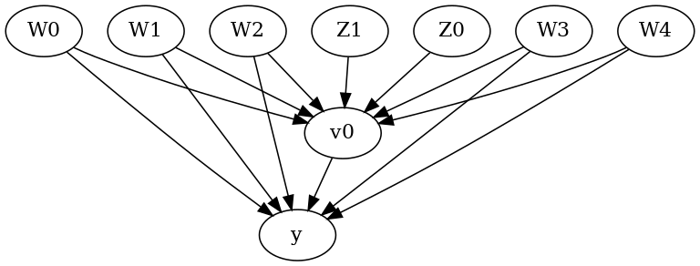
We get a causal graph. Now identification and estimation is done.
[7]:
identified_estimand = model.identify_effect(proceed_when_unidentifiable=True)
print(identified_estimand)
Estimand type: EstimandType.NONPARAMETRIC_ATE

### Estimand : 1
Estimand name: backdoor
Estimand expression:
  d
─────(E[y|W2,W3,W0,W4,W1])
d[v₀]
Estimand assumption 1, Unconfoundedness: If U→{v0} and U→y then P(y|v0,W2,W3,W0,W4,W1,U) = P(y|v0,W2,W3,W0,W4,W1)

### Estimand : 2
Estimand name: iv
Estimand expression:
 ⎡                              -1⎤
 ⎢    d        ⎛    d          ⎞  ⎥
E⎢─────────(y)⋅⎜─────────([v₀])⎟  ⎥
 ⎣d[Z₀  Z₁]    ⎝d[Z₀  Z₁]      ⎠  ⎦
Estimand assumption 1, As-if-random: If U→→y then ¬(U →→{Z0,Z1})
Estimand assumption 2, Exclusion: If we remove {Z0,Z1}→{v0}, then ¬({Z0,Z1}→y)

### Estimand : 3
Estimand name: frontdoor
No such variable(s) found!
Method 1: Regression
Use linear regression.
[8]:
causal_estimate_reg = model.estimate_effect(identified_estimand,
        method_name="backdoor.linear_regression",
        test_significance=True)
print(causal_estimate_reg)
print("Causal Estimate is " + str(causal_estimate_reg.value))
*** Causal Estimate ***

## Identified estimand
Estimand type: EstimandType.NONPARAMETRIC_ATE

### Estimand : 1
Estimand name: backdoor
Estimand expression:
  d
─────(E[y|W2,W3,W0,W4,W1])
d[v₀]
Estimand assumption 1, Unconfoundedness: If U→{v0} and U→y then P(y|v0,W2,W3,W0,W4,W1,U) = P(y|v0,W2,W3,W0,W4,W1)

## Realized estimand
b: y~v0+W2+W3+W0+W4+W1
Target units: ate

## Estimate
Mean value: 10.00010276682088

Causal Estimate is 10.00010276682088
Method 2: Distance Matching
Define a distance metric and then use the metric to match closest points between treatment and control.
[9]:
causal_estimate_dmatch = model.estimate_effect(identified_estimand,
                                              method_name="backdoor.distance_matching",
                                              target_units="att",
                                              method_params={'distance_metric':"minkowski", 'p':2})
print(causal_estimate_dmatch)
print("Causal Estimate is " + str(causal_estimate_dmatch.value))
*** Causal Estimate ***

## Identified estimand
Estimand type: EstimandType.NONPARAMETRIC_ATE

### Estimand : 1
Estimand name: backdoor
Estimand expression:
  d
─────(E[y|W2,W3,W0,W4,W1])
d[v₀]
Estimand assumption 1, Unconfoundedness: If U→{v0} and U→y then P(y|v0,W2,W3,W0,W4,W1,U) = P(y|v0,W2,W3,W0,W4,W1)

## Realized estimand
b: y~v0+W2+W3+W0+W4+W1
Target units: att

## Estimate
Mean value: 10.503493860521266

Causal Estimate is 10.503493860521266
Method 3: Propensity Score Stratification
We will be using propensity scores to stratify units in the data.
[10]:
causal_estimate_strat = model.estimate_effect(identified_estimand,
                                              method_name="backdoor.propensity_score_stratification",
                                              target_units="att")
print(causal_estimate_strat)
print("Causal Estimate is " + str(causal_estimate_strat.value))
*** Causal Estimate ***

## Identified estimand
Estimand type: EstimandType.NONPARAMETRIC_ATE

### Estimand : 1
Estimand name: backdoor
Estimand expression:
  d
─────(E[y|W2,W3,W0,W4,W1])
d[v₀]
Estimand assumption 1, Unconfoundedness: If U→{v0} and U→y then P(y|v0,W2,W3,W0,W4,W1,U) = P(y|v0,W2,W3,W0,W4,W1)

## Realized estimand
b: y~v0+W2+W3+W0+W4+W1
Target units: att

## Estimate
Mean value: 9.874113053820228

Causal Estimate is 9.874113053820228
Method 4: Propensity Score Matching
We will be using propensity scores to match units in the data.
[11]:
causal_estimate_match = model.estimate_effect(identified_estimand,
                                              method_name="backdoor.propensity_score_matching",
                                              target_units="atc")
print(causal_estimate_match)
print("Causal Estimate is " + str(causal_estimate_match.value))
*** Causal Estimate ***

## Identified estimand
Estimand type: EstimandType.NONPARAMETRIC_ATE

### Estimand : 1
Estimand name: backdoor
Estimand expression:
  d
─────(E[y|W2,W3,W0,W4,W1])
d[v₀]
Estimand assumption 1, Unconfoundedness: If U→{v0} and U→y then P(y|v0,W2,W3,W0,W4,W1,U) = P(y|v0,W2,W3,W0,W4,W1)

## Realized estimand
b: y~v0+W2+W3+W0+W4+W1
Target units: atc

## Estimate
Mean value: 9.89316687854654

Causal Estimate is 9.89316687854654
Method 5: Weighting
We will be using (inverse) propensity scores to assign weights to units in the data. DoWhy supports a few different weighting schemes: 1. Vanilla Inverse Propensity Score weighting (IPS) (weighting_scheme=“ips_weight”) 2. Self-normalized IPS weighting (also known as the Hajek estimator) (weighting_scheme=“ips_normalized_weight”) 3. Stabilized IPS weighting (weighting_scheme = “ips_stabilized_weight”)
[12]:
causal_estimate_ipw = model.estimate_effect(identified_estimand,
                                            method_name="backdoor.propensity_score_weighting",
                                            target_units = "ate",
                                            method_params={"weighting_scheme":"ips_weight"})
print(causal_estimate_ipw)
print("Causal Estimate is " + str(causal_estimate_ipw.value))
*** Causal Estimate ***

## Identified estimand
Estimand type: EstimandType.NONPARAMETRIC_ATE

### Estimand : 1
Estimand name: backdoor
Estimand expression:
  d
─────(E[y|W2,W3,W0,W4,W1])
d[v₀]
Estimand assumption 1, Unconfoundedness: If U→{v0} and U→y then P(y|v0,W2,W3,W0,W4,W1,U) = P(y|v0,W2,W3,W0,W4,W1)

## Realized estimand
b: y~v0+W2+W3+W0+W4+W1
Target units: ate

## Estimate
Mean value: 11.019679871018909

Causal Estimate is 11.019679871018909
Method 6: Instrumental Variable
We will be using the Wald estimator for the provided instrumental variable.
[13]:
causal_estimate_iv = model.estimate_effect(identified_estimand,
        method_name="iv.instrumental_variable", method_params = {'iv_instrument_name': 'Z0'})
print(causal_estimate_iv)
print("Causal Estimate is " + str(causal_estimate_iv.value))
*** Causal Estimate ***

## Identified estimand
Estimand type: EstimandType.NONPARAMETRIC_ATE

### Estimand : 1
Estimand name: iv
Estimand expression:
 ⎡                              -1⎤
 ⎢    d        ⎛    d          ⎞  ⎥
E⎢─────────(y)⋅⎜─────────([v₀])⎟  ⎥
 ⎣d[Z₀  Z₁]    ⎝d[Z₀  Z₁]      ⎠  ⎦
Estimand assumption 1, As-if-random: If U→→y then ¬(U →→{Z0,Z1})
Estimand assumption 2, Exclusion: If we remove {Z0,Z1}→{v0}, then ¬({Z0,Z1}→y)

## Realized estimand
Realized estimand: Wald Estimator
Realized estimand type: EstimandType.NONPARAMETRIC_ATE
Estimand expression:
 ⎡ d    ⎤  -1⎡ d     ⎤
E⎢───(y)⎥⋅E  ⎢───(v₀)⎥
 ⎣dZ₀   ⎦    ⎣dZ₀    ⎦
Estimand assumption 1, As-if-random: If U→→y then ¬(U →→{Z0,Z1})
Estimand assumption 2, Exclusion: If we remove {Z0,Z1}→{v0}, then ¬({Z0,Z1}→y)
Estimand assumption 3, treatment_effect_homogeneity: Each unit's treatment ['v0'] is affected in the same way by common causes of ['v0'] and y
Estimand assumption 4, outcome_effect_homogeneity: Each unit's outcome y is affected in the same way by common causes of ['v0'] and y

Target units: ate

## Estimate
Mean value: 10.292005072827397

Causal Estimate is 10.292005072827397
Method 7: Regression Discontinuity
We will be internally converting this to an equivalent instrumental variables problem.
[14]:
causal_estimate_regdist = model.estimate_effect(identified_estimand,
        method_name="iv.regression_discontinuity",
        method_params={'rd_variable_name':'Z1',
                       'rd_threshold_value':0.5,
                       'rd_bandwidth': 0.15})
print(causal_estimate_regdist)
print("Causal Estimate is " + str(causal_estimate_regdist.value))
*** Causal Estimate ***

## Identified estimand
Estimand type: EstimandType.NONPARAMETRIC_ATE

### Estimand : 1
Estimand name: iv
Estimand expression:
 ⎡                              -1⎤
 ⎢    d        ⎛    d          ⎞  ⎥
E⎢─────────(y)⋅⎜─────────([v₀])⎟  ⎥
 ⎣d[Z₀  Z₁]    ⎝d[Z₀  Z₁]      ⎠  ⎦
Estimand assumption 1, As-if-random: If U→→y then ¬(U →→{Z0,Z1})
Estimand assumption 2, Exclusion: If we remove {Z0,Z1}→{v0}, then ¬({Z0,Z1}→y)

## Realized estimand
Realized estimand: Wald Estimator
Realized estimand type: EstimandType.NONPARAMETRIC_ATE
Estimand expression:
 ⎡        d            ⎤  -1⎡        d             ⎤
E⎢──────────────────(y)⎥⋅E  ⎢──────────────────(v₀)⎥
 ⎣dlocal_rd_variable   ⎦    ⎣dlocal_rd_variable    ⎦
Estimand assumption 1, As-if-random: If U→→y then ¬(U →→{Z0,Z1})
Estimand assumption 2, Exclusion: If we remove {Z0,Z1}→{v0}, then ¬({Z0,Z1}→y)
Estimand assumption 3, treatment_effect_homogeneity: Each unit's treatment ['local_treatment'] is affected in the same way by common causes of ['local_treatment'] and local_outcome
Estimand assumption 4, outcome_effect_homogeneity: Each unit's outcome local_outcome is affected in the same way by common causes of ['local_treatment'] and local_outcome

Target units: ate

## Estimate
Mean value: 12.042026081818154

Causal Estimate is 12.042026081818154