DoWhy example on the Lalonde dataset

Thanks to [@mizuy](https://github.com/mizuy) for providing this example. Here we use the Lalonde dataset and apply IPW estimator to it.

1. Load the data

import dowhy.datasets

lalonde = dowhy.datasets.lalonde_dataset()

2. Run DoWhy analysis: model, identify, estimate

from dowhy import CausalModel


model=CausalModel(
        data = lalonde,
        treatment='treat',
        outcome='re78',
        common_causes='nodegr+black+hisp+age+educ+married'.split('+'))
identified_estimand = model.identify_effect(proceed_when_unidentifiable=True)
estimate = model.estimate_effect(identified_estimand,
        method_name="backdoor.propensity_score_weighting",
        target_units="ate",
        method_params={"weighting_scheme":"ips_weight"})

print("Causal Estimate is " + str(estimate.value))

import statsmodels.formula.api as smf
reg=smf.wls('re78~1+treat', data=lalonde, weights=lalonde.ips_stabilized_weight)
res=reg.fit()
res.summary()

Causal Estimate is 1639.8096006295063

WLS Regression Results

Dep. Variable:	re78	R-squared:	0.015
Model:	WLS	Adj. R-squared:	0.013
Method:	Least Squares	F-statistic:	6.743
Date:	Sat, 17 Dec 2022	Prob (F-statistic):	0.00973
Time:	06:41:56	Log-Likelihood:	-4544.7
No. Observations:	445	AIC:	9093.
Df Residuals:	443	BIC:	9102.
Df Model:	1
Covariance Type:	nonrobust

	coef	std err	t	P>|t|	[0.025	0.975]
Intercept	4555.0743	406.704	11.200	0.000	3755.765	5354.383
treat[T.True]	1639.8096	631.496	2.597	0.010	398.710	2880.909

Omnibus:	303.263	Durbin-Watson:	2.085
Prob(Omnibus):	0.000	Jarque-Bera (JB):	4770.626
Skew:	2.709	Prob(JB):	0.00
Kurtosis:	18.097	Cond. No.	2.47

Notes:
[1] Standard Errors assume that the covariance matrix of the errors is correctly specified.

3. Interpret the estimate

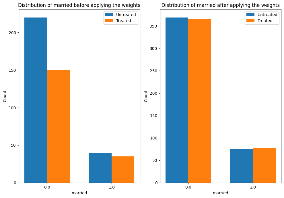
The plot below shows how the distribution of a confounder, “married” changes from the original data to the weighted data. In both datasets, we compare the distribution of “married” across treated and untreated units.

estimate.interpret(method_name="confounder_distribution_interpreter",var_type='discrete',
                   var_name='married', fig_size = (10, 7), font_size = 12)

4. Sanity check: compare to manual IPW estimate

df = model._data
ps = df['propensity_score']
y = df['re78']
z = df['treat']

ey1 = z*y/ps / sum(z/ps)
ey0 = (1-z)*y/(1-ps) / sum((1-z)/(1-ps))
ate = ey1.sum()-ey0.sum()
print("Causal Estimate is " + str(ate))

# correct -> Causal Estimate is 1634.9868359746906

Causal Estimate is 1639.8096006295073