Conditional Average Treatment Effects (CATE) with DoWhy and EconML
This is an experimental feature where we use EconML methods from DoWhy. Using EconML allows CATE estimation using different methods.
All four steps of causal inference in DoWhy remain the same: model, identify, estimate, and refute. The key difference is that we now call econml methods in the estimation step. There is also a simpler example using linear regression to understand the intuition behind CATE estimators.
All datasets are generated using linear structural equations.
[1]:
%load_ext autoreload
%autoreload 2
[2]:
import numpy as np
import pandas as pd
import logging

import dowhy
from dowhy import CausalModel
import dowhy.datasets

import econml
import warnings
warnings.filterwarnings('ignore')

BETA = 10
[3]:
data = dowhy.datasets.linear_dataset(BETA, num_common_causes=4, num_samples=10000,
                                    num_instruments=2, num_effect_modifiers=2,
                                     num_treatments=1,
                                    treatment_is_binary=False,
                                    num_discrete_common_causes=2,
                                    num_discrete_effect_modifiers=0,
                                    one_hot_encode=False)
df=data['df']
print(df.head())
print("True causal estimate is", data["ate"])
         X0        X1   Z0        Z1        W0        W1 W2 W3         v0  \
0 -0.231749 -0.231050  0.0  0.432344 -0.114830  0.116381  2  1   6.097601
1  1.325174 -1.080612  0.0  0.929593 -0.726349  0.076760  3  1  10.194262
2  0.204770 -0.415769  0.0  0.288978 -1.471662 -2.507972  1  3  -1.720668
3 -1.401098  0.231546  0.0  0.851559 -0.936729  0.998402  1  3  10.684910
4 -0.371536 -0.477363  0.0  0.464857 -2.156732  1.736986  2  0   1.652021

            y
0   64.992364
1   86.274053
2  -11.504137
3  118.478051
4   20.976498
True causal estimate is 7.0157725790875745
[4]:
model = CausalModel(data=data["df"],
                    treatment=data["treatment_name"], outcome=data["outcome_name"],
                    graph=data["gml_graph"])
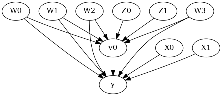
[5]:
model.view_model()
from IPython.display import Image, display
display(Image(filename="causal_model.png"))
[6]:
identified_estimand= model.identify_effect(proceed_when_unidentifiable=True)
print(identified_estimand)
Estimand type: EstimandType.NONPARAMETRIC_ATE

### Estimand : 1
Estimand name: backdoor
Estimand expression:
  d
─────(E[y|W2,W1,W3,W0])
d[v₀]
Estimand assumption 1, Unconfoundedness: If U→{v0} and U→y then P(y|v0,W2,W1,W3,W0,U) = P(y|v0,W2,W1,W3,W0)

### Estimand : 2
Estimand name: iv
Estimand expression:
 ⎡                              -1⎤
 ⎢    d        ⎛    d          ⎞  ⎥
E⎢─────────(y)⋅⎜─────────([v₀])⎟  ⎥
 ⎣d[Z₁  Z₀]    ⎝d[Z₁  Z₀]      ⎠  ⎦
Estimand assumption 1, As-if-random: If U→→y then ¬(U →→{Z1,Z0})
Estimand assumption 2, Exclusion: If we remove {Z1,Z0}→{v0}, then ¬({Z1,Z0}→y)

### Estimand : 3
Estimand name: frontdoor
No such variable(s) found!
Linear Model
First, let us build some intuition using a linear model for estimating CATE. The effect modifiers (that lead to a heterogeneous treatment effect) can be modeled as interaction terms with the treatment. Thus, their value modulates the effect of treatment.
Below the estimated effect of changing treatment from 0 to 1.
[7]:
linear_estimate = model.estimate_effect(identified_estimand,
                                        method_name="backdoor.linear_regression",
                                       control_value=0,
                                       treatment_value=1)
print(linear_estimate)
*** Causal Estimate ***

## Identified estimand
Estimand type: EstimandType.NONPARAMETRIC_ATE

### Estimand : 1
Estimand name: backdoor
Estimand expression:
  d
─────(E[y|W2,W1,W3,W0])
d[v₀]
Estimand assumption 1, Unconfoundedness: If U→{v0} and U→y then P(y|v0,W2,W1,W3,W0,U) = P(y|v0,W2,W1,W3,W0)

## Realized estimand
b: y~v0+W2+W1+W3+W0+v0*X1+v0*X0
Target units: ate

## Estimate
Mean value: 7.015522453946055
EconML methods
We now move to the more advanced methods from the EconML package for estimating CATE.
First, let us look at the double machine learning estimator. Method_name corresponds to the fully qualified name of the class that we want to use. For double ML, it is “econml.dml.DML”.
Target units defines the units over which the causal estimate is to be computed. This can be a lambda function filter on the original dataframe, a new Pandas dataframe, or a string corresponding to the three main kinds of target units (“ate”, “att” and “atc”). Below we show an example of a lambda function.
Method_params are passed directly to EconML. For details on allowed parameters, refer to the EconML documentation.
[8]:
from sklearn.preprocessing import PolynomialFeatures
from sklearn.linear_model import LassoCV
from sklearn.ensemble import GradientBoostingRegressor
dml_estimate = model.estimate_effect(identified_estimand, method_name="backdoor.econml.dml.DML",
                                     control_value = 0,
                                     treatment_value = 1,
                                 target_units = lambda df: df["X0"]>1,  # condition used for CATE
                                 confidence_intervals=False,
                                method_params={"init_params":{'model_y':GradientBoostingRegressor(),
                                                              'model_t': GradientBoostingRegressor(),
                                                              "model_final":LassoCV(fit_intercept=False),
                                                              'featurizer':PolynomialFeatures(degree=1, include_bias=False)},
                                               "fit_params":{}})
print(dml_estimate)
*** Causal Estimate ***

## Identified estimand
Estimand type: EstimandType.NONPARAMETRIC_ATE

### Estimand : 1
Estimand name: backdoor
Estimand expression:
  d
─────(E[y|W2,W1,W3,W0])
d[v₀]
Estimand assumption 1, Unconfoundedness: If U→{v0} and U→y then P(y|v0,W2,W1,W3,W0,U) = P(y|v0,W2,W1,W3,W0)

## Realized estimand
b: y~v0+W2+W1+W3+W0 | X1,X0
Target units: Data subset defined by a function

## Estimate
Mean value: 8.832955504861756
Effect estimates: [[ 7.15809974]
 [ 8.23425738]
 [ 9.17911651]
 [ 2.31152959]
 [ 4.87413987]
 [13.88945749]
 [ 7.48876631]
 [13.49191116]
 [ 9.901151  ]
 [ 9.51314013]
 [11.21696872]
 [13.82425142]
 [ 8.84875949]
 [11.48307094]
 [ 7.62409547]
 [ 4.81389901]
 [ 8.69728372]
 [ 6.7418683 ]
 [ 9.97080827]
 [13.26662522]
 [ 6.62479954]
 [ 9.67326911]
 [ 6.15092419]
 [10.08013496]
 [ 7.16475572]
 [ 9.61003886]
 [12.05548322]
 [ 7.09182211]
 [14.18258511]
 [ 9.88070794]
 [10.04725786]
 [ 8.8006271 ]
 [16.77507642]
 [11.2338629 ]
 [12.34420786]
 [ 7.42868003]
 [ 8.34474036]
 [ 6.38138818]
 [ 3.3121635 ]
 [ 7.11443635]
 [ 6.12408273]
 [14.90273937]
 [ 4.97171895]
 [12.31507859]
 [ 6.62868179]
 [13.89775238]
 [ 3.36002293]
 [ 4.82092936]
 [13.2814885 ]
 [ 3.7016386 ]
 [ 7.40705642]
 [ 9.02297757]
 [ 8.90356146]
 [10.13097341]
 [ 8.84136361]
 [ 7.31129423]
 [ 7.85532657]
 [ 9.88852709]
 [10.50544746]
 [ 7.35448063]
 [ 4.06871203]
 [15.34910472]
 [14.07965081]
 [ 9.31242049]
 [ 5.74090827]
 [ 8.06160171]
 [ 6.84948804]
 [ 3.55456605]
 [ 9.48659929]
 [13.03589279]
 [15.90202301]
 [ 8.75951122]
 [12.71974757]
 [ 7.80153869]
 [ 9.82068702]
 [14.75734993]
 [ 3.28526897]
 [12.45193185]
 [11.85338007]
 [13.74123704]
 [ 0.17538186]
 [ 6.18269855]
 [ 4.97329517]
 [ 5.77106175]
 [ 7.19236445]
 [11.3748272 ]
 [ 9.54652898]
 [15.29059804]
 [ 9.24540153]
 [ 6.85568096]
 [15.55056995]
 [ 3.83873451]
 [ 6.90683139]
 [11.88671678]
 [ 8.82637317]
 [ 7.93826922]
 [ 7.0378285 ]
 [17.67062573]
 [11.81918835]
 [ 7.08951273]
 [15.6796889 ]
 [ 4.01106311]
 [ 9.62641457]
 [ 0.73637794]
 [ 8.02876557]
 [ 4.89218164]
 [11.28112768]
 [ 9.8490302 ]
 [ 7.14682889]
 [13.73347838]
 [-0.99187172]
 [12.12255092]
 [ 8.32662435]
 [ 4.87523226]
 [12.91793162]
 [ 7.43005683]
 [ 1.35872222]
 [ 9.25565376]
 [10.93571261]
 [ 6.1171659 ]
 [ 6.50302008]
 [11.16804571]
 [ 3.95112634]
 [ 8.56010137]
 [11.09137866]
 [12.32462446]
 [12.08581428]
 [11.11162852]
 [14.5648803 ]
 [ 5.33512882]
 [13.5846904 ]
 [10.38868967]
 [ 7.93555617]
 [ 6.93400055]
 [ 8.48251096]
 [ 1.04091425]
 [ 9.98243191]
 [ 8.23472158]
 [ 3.25634578]
 [ 6.35908316]
 [10.9968092 ]
 [12.02244309]
 [ 5.80220424]
 [ 9.69153941]
 [ 9.68126719]
 [ 6.7297331 ]
 [ 5.0162273 ]
 [13.68921589]
 [ 6.97227711]
 [ 9.04775005]
 [ 9.0836503 ]
 [16.01695511]
 [11.19883022]
 [ 8.8634017 ]
 [10.7428037 ]
 [ 9.8654083 ]
 [ 3.17285288]
 [ 3.71555135]
 [ 5.3015171 ]
 [ 7.21226999]
 [ 6.76429005]
 [18.57625508]
 [15.80853322]
 [10.77282488]
 [10.97115821]
 [ 7.83219437]
 [10.17415394]
 [16.05282323]
 [ 9.67822897]
 [ 6.56858607]
 [15.61842606]
 [12.67147045]
 [10.17065183]
 [13.0857411 ]
 [ 6.15178442]
 [ 5.88467642]
 [ 4.93783059]
 [ 3.61466595]
 [ 2.3044093 ]
 [ 7.75381584]
 [ 8.5949979 ]
 [16.23991468]
 [10.68244865]
 [ 9.43889147]
 [ 3.77258878]
 [10.75280018]
 [ 6.78064259]
 [11.33554799]
 [ 8.14170212]
 [ 5.09164985]
 [14.62581648]
 [13.17065734]
 [15.20398894]
 [ 8.28782285]
 [13.49419811]
 [ 9.04632635]
 [ 6.52207808]
 [15.18214291]
 [ 5.65477641]
 [11.03036519]
 [14.81450638]
 [ 6.47812136]
 [ 8.24949237]
 [ 8.39909305]
 [ 2.46276264]
 [ 2.96599403]
 [ 2.09321384]
 [11.66944326]
 [ 6.09293032]
 [ 3.38728989]
 [15.35379975]
 [13.94112497]
 [ 8.14491184]
 [ 1.83590725]
 [-0.35161247]
 [ 9.25257547]
 [ 5.50123953]
 [ 5.45949069]
 [ 8.59042845]
 [ 3.90861362]
 [11.62956379]
 [ 9.77325941]
 [ 9.26884606]
 [15.87167299]
 [ 2.72868926]
 [11.97383857]
 [ 8.58518235]
 [10.84067264]
 [18.67135503]
 [12.3498595 ]
 [ 3.59725782]
 [11.6974085 ]
 [12.47366077]
 [ 5.79023854]
 [ 8.87612845]
 [ 6.61809686]
 [ 1.41237672]
 [ 6.74846069]
 [ 3.75487661]
 [12.92108707]
 [ 8.10074003]
 [ 5.00091793]
 [ 7.13077751]
 [ 7.50921405]
 [ 4.71040862]
 [ 8.83543095]
 [ 7.06225146]
 [ 4.89383011]
 [ 6.89385468]
 [12.35823033]
 [10.19688593]
 [-0.17219868]
 [16.82529767]
 [ 7.14949324]
 [ 7.406859  ]
 [ 4.27421337]
 [ 8.99322567]
 [ 9.82273464]
 [11.20524278]
 [10.02666378]
 [ 1.16294873]
 [11.74423489]
 [11.09901931]
 [12.61762271]
 [ 7.37145124]
 [12.6639333 ]
 [ 7.94634305]
 [12.37155568]
 [15.31699491]
 [ 9.50296573]
 [-0.1757215 ]
 [11.21172109]
 [15.46336452]
 [ 9.82913498]
 [ 9.207347  ]
 [ 7.42289828]
 [ 7.65440316]
 [ 9.8452771 ]
 [ 9.6173368 ]
 [14.55031049]
 [ 8.6304493 ]
 [10.31774684]
 [11.63934296]
 [10.19497905]
 [ 7.77213878]
 [10.74969258]
 [10.32364223]
 [ 5.55215163]
 [ 2.32458977]
 [ 4.04470881]
 [ 7.13941054]
 [11.2694548 ]
 [ 7.77244792]
 [12.9224708 ]
 [ 9.12581443]
 [15.57353661]
 [ 7.60862983]
 [ 9.16347198]
 [ 7.76391752]
 [11.74747905]
 [ 5.74164525]
 [ 4.512569  ]
 [ 7.39607696]
 [ 6.42345107]
 [10.38747374]
 [ 8.12014851]
 [ 9.92187468]
 [ 2.54611921]
 [ 6.12554917]
 [14.37147299]
 [ 4.37701739]
 [ 8.26338418]
 [19.2194248 ]
 [11.90663915]
 [ 6.95078213]
 [10.35831565]
 [ 6.60834329]
 [-0.13997248]
 [ 6.9851859 ]
 [15.12171917]
 [14.78759619]
 [14.97643547]
 [11.03427713]
 [ 9.04890747]
 [12.34458812]
 [13.54111133]
 [ 7.45832533]
 [ 1.6064396 ]
 [ 7.33044281]
 [ 8.11742225]
 [10.59702862]
 [ 8.01179899]
 [15.8730726 ]
 [ 7.36621074]
 [ 4.33249031]
 [ 8.27296941]
 [ 9.43895063]
 [ 1.24293911]
 [ 7.66890002]
 [ 6.05436377]
 [ 5.52740003]
 [11.09864381]
 [16.3899675 ]
 [ 7.55906235]
 [ 5.72041966]
 [ 5.57314658]
 [ 6.13369401]
 [10.88272187]
 [11.76106025]
 [10.34376597]
 [10.16117524]
 [ 9.23191658]
 [ 8.55083594]
 [ 5.02165889]
 [ 4.79527397]
 [ 8.16052432]
 [12.92506041]
 [13.93760408]
 [ 8.05687284]
 [ 2.87306396]
 [ 8.3033085 ]
 [ 6.08158909]
 [ 9.65968217]
 [ 3.15628006]
 [ 9.79144221]
 [ 5.45026107]
 [-0.06908761]
 [10.36381734]
 [12.20627059]
 [ 7.01799995]
 [ 6.12796752]
 [ 7.07296223]
 [ 3.67130015]
 [ 7.7805081 ]
 [11.13051312]
 [ 7.76530823]
 [ 1.55108882]
 [12.13241796]
 [ 3.35685043]
 [11.14131481]
 [15.71640511]
 [ 4.65578484]
 [ 6.02856182]
 [ 4.49734387]
 [ 7.30118531]
 [ 3.78647712]
 [12.01934208]
 [ 4.84714621]
 [ 9.59042571]
 [ 5.91837718]
 [12.49177556]
 [ 7.55875231]
 [ 6.81810706]
 [ 7.50579304]
 [ 4.49041292]
 [ 9.29225674]
 [ 8.79535932]
 [ 7.66879774]
 [ 8.56584243]
 [13.66270772]
 [ 1.79643322]
 [11.82866164]
 [ 7.35922342]
 [ 4.55133016]
 [13.4866857 ]
 [-0.34435079]
 [10.40953492]
 [ 9.62764837]
 [12.67887629]
 [10.39720693]
 [10.87661318]
 [11.73889149]
 [ 8.74776528]
 [11.25920874]
 [ 1.66781537]
 [ 5.40884061]
 [11.37662653]
 [ 9.01400614]
 [ 3.04961239]
 [11.99851992]
 [10.95043927]
 [13.69651669]
 [11.47656825]
 [ 3.81975483]
 [10.1991278 ]
 [ 6.40604012]
 [ 7.73334398]
 [ 2.87462062]
 [ 2.96363035]
 [10.47437861]
 [ 6.46822858]
 [ 9.77654877]
 [15.77266062]
 [17.29584454]
 [12.50973717]
 [ 6.63802846]
 [ 5.16285218]
 [ 4.8470301 ]
 [ 7.95752508]
 [ 1.05324541]
 [12.33083235]
 [ 7.32991936]
 [ 6.98071474]
 [13.44506773]
 [10.70868399]
 [ 9.38827026]
 [ 7.61221758]
 [13.71275537]
 [ 9.27260429]
 [ 5.78999256]
 [ 8.09064027]
 [ 5.90339691]
 [12.18410367]
 [ 9.04144752]
 [10.14737614]
 [16.5936071 ]
 [ 7.21244931]
 [ 7.30795132]
 [12.00664627]
 [ 6.34115143]
 [10.46794723]
 [ 2.89488563]
 [ 8.16486677]
 [11.91293599]
 [ 6.66677793]
 [ 5.5732688 ]
 [ 7.55500507]
 [ 6.80208011]
 [ 9.62018113]
 [13.90507652]
 [10.22698582]
 [ 4.44134999]
 [11.92248853]
 [ 7.59204934]
 [ 0.11220069]
 [ 6.27300038]
 [ 5.027799  ]
 [ 8.24724878]
 [ 8.89755155]
 [13.40141484]
 [ 5.80727332]
 [10.31799888]
 [11.54083443]
 [15.59615814]
 [ 3.2421135 ]
 [ 3.91726011]
 [11.78705913]
 [ 8.85110709]
 [ 6.7668797 ]
 [ 8.11451884]
 [ 3.38499519]
 [ 3.4176808 ]
 [10.91133649]
 [17.57506377]
 [14.20998411]
 [10.16357339]
 [10.04666003]
 [ 7.27220246]
 [ 6.1452778 ]
 [ 5.54822926]
 [11.48243795]
 [ 9.45018434]
 [10.98995067]
 [12.31813444]
 [ 9.16163588]
 [ 9.49089268]
 [ 8.25250051]
 [ 8.31500374]
 [ 5.8363085 ]
 [ 4.26774178]
 [ 9.49778358]
 [ 7.18016876]
 [17.9184414 ]
 [ 6.12452336]
 [ 5.89426567]
 [10.67821307]
 [11.75791173]
 [ 9.7980118 ]
 [ 8.15030047]
 [12.52480085]
 [ 7.24277214]
 [ 9.72511085]
 [ 7.53044555]
 [ 7.83437505]
 [ 3.23295906]
 [10.38947862]
 [ 9.59703551]
 [ 5.30688369]
 [ 8.195482  ]
 [ 8.7490108 ]
 [ 5.24474988]
 [11.37984416]
 [ 8.29800562]
 [11.19744182]
 [11.65527311]
 [ 4.77513079]
 [ 0.6748703 ]
 [ 3.91118804]
 [ 8.53496142]
 [ 2.35356213]
 [10.78974633]
 [ 7.38671953]
 [ 8.50616827]
 [11.20968689]
 [ 3.27700853]
 [ 6.76941268]
 [13.32451586]
 [ 7.46495288]
 [13.02318118]
 [ 8.35758863]
 [ 6.28996323]
 [ 4.7493668 ]
 [ 6.14614607]
 [ 2.77707663]
 [ 2.46361093]
 [ 5.79247711]
 [ 5.03987818]
 [14.09466324]
 [ 7.47814559]
 [10.35237235]
 [ 4.56728269]
 [10.1157313 ]
 [ 4.53924423]
 [ 3.0012394 ]
 [13.00499115]
 [12.93608838]
 [ 5.7755288 ]
 [ 8.54974394]
 [12.7646931 ]
 [16.67298008]
 [ 7.9908849 ]
 [11.0426114 ]
 [10.50710246]
 [ 7.09998527]
 [ 7.8001349 ]
 [11.69492114]
 [12.60367377]
 [ 2.97195028]
 [13.26770266]
 [11.56201134]
 [11.59828173]
 [10.88448882]
 [ 9.81670711]
 [ 8.55350215]
 [14.03976822]
 [13.45930873]
 [13.31293426]
 [ 6.64035775]
 [13.2118298 ]
 [ 6.92254276]
 [11.27506987]
 [16.78123301]
 [-0.76540665]
 [14.17790894]
 [ 2.49349703]
 [ 8.85201396]
 [ 7.82339891]
 [12.81439053]
 [14.26369888]
 [ 4.25897277]
 [ 8.64634229]
 [ 6.97467195]
 [-1.61449562]
 [ 9.60106769]
 [ 7.91490433]
 [ 8.42246677]
 [10.0298052 ]
 [ 5.96569484]
 [11.58266472]
 [11.419268  ]
 [ 7.91047724]
 [11.21668648]
 [10.55217224]
 [10.26432219]
 [ 7.8941198 ]
 [ 4.59605379]
 [11.9955753 ]
 [ 2.82398053]
 [ 7.19428101]
 [11.4770032 ]
 [ 8.31584464]
 [ 7.23400945]
 [ 8.27898216]
 [ 6.24508983]
 [10.32638494]
 [ 9.78038913]
 [ 7.39720009]
 [ 7.27122739]
 [10.83762804]
 [10.00821887]
 [ 7.47100721]
 [ 7.98060664]
 [ 8.49625109]
 [11.52020616]
 [-1.77922802]
 [14.05158298]
 [15.28088974]
 [ 9.37937437]
 [ 8.0595868 ]
 [ 7.76306776]
 [10.69559967]
 [ 8.06245009]
 [11.04258249]
 [10.56124832]
 [ 7.39896028]
 [13.36454114]
 [ 8.68145883]
 [10.21827325]
 [10.85054894]
 [14.22788722]
 [11.82145104]
 [ 7.55276143]
 [14.10552402]
 [10.11443285]
 [12.93084328]
 [ 2.53410359]
 [ 5.38071421]
 [12.93045189]
 [14.84772505]
 [ 5.76197256]
 [11.03684456]
 [ 7.54001963]
 [11.41489298]
 [ 4.47755414]
 [10.9477281 ]
 [ 6.07608793]
 [ 6.8856347 ]
 [ 9.65476862]
 [ 9.63556619]
 [12.45000029]
 [ 2.84392277]
 [12.39965805]
 [ 6.82170322]
 [ 7.10855002]
 [ 5.87454474]
 [12.40204126]
 [11.16624038]
 [ 6.60316648]
 [12.06810928]
 [ 6.12200746]
 [ 6.08203993]
 [ 6.51110229]
 [ 9.05728024]
 [12.07885093]
 [ 8.87465977]
 [12.91570811]
 [ 8.34176758]
 [ 7.77620637]
 [ 7.44465255]
 [14.06763302]
 [ 9.95356284]
 [ 9.97416191]
 [ 4.65294468]
 [ 7.12678795]
 [ 9.76012541]
 [ 8.02432823]
 [ 5.6988445 ]
 [16.04515159]
 [12.35733149]
 [ 1.18021564]
 [10.32431306]
 [ 9.0039998 ]
 [14.69099459]
 [12.38399276]
 [ 9.6841394 ]
 [11.26426245]
 [11.38206564]
 [14.52533772]
 [ 8.22008586]
 [ 7.59179905]
 [ 4.88407166]
 [12.11262723]
 [ 7.8880226 ]
 [ 9.75681719]
 [ 8.21539157]
 [ 9.42653877]
 [13.38404394]
 [ 5.69706273]
 [13.69005331]
 [14.73628812]
 [ 7.54998804]
 [10.34792839]
 [ 6.32389367]
 [12.52666801]
 [16.91737062]
 [10.0167292 ]
 [ 7.15012531]
 [ 2.6509039 ]
 [10.54525463]
 [15.71114207]
 [ 6.67398479]
 [ 3.67580423]
 [14.46161829]
 [ 6.82023285]
 [14.03333625]
 [ 9.13348557]
 [ 9.70626158]
 [ 8.5728083 ]
 [ 4.5777442 ]
 [ 2.18069258]
 [14.19801145]
 [ 4.2574885 ]
 [-1.60306499]
 [18.17686081]
 [ 8.99894712]
 [ 7.69849072]
 [13.12474633]
 [ 8.32248211]
 [ 7.89632652]
 [ 8.83910356]
 [14.48421063]
 [12.38309781]
 [ 7.78067858]
 [14.84016956]
 [12.73956515]
 [ 9.62529926]
 [ 2.3615847 ]
 [ 1.25850672]
 [ 7.47025827]
 [10.17022903]
 [13.77347795]
 [ 1.86010844]
 [-2.13878698]
 [16.26021293]
 [12.77123591]
 [13.26249453]
 [ 5.29209754]
 [ 9.15182784]
 [14.15243309]
 [ 9.52557545]
 [ 7.34045783]
 [ 4.98613201]
 [ 7.29348545]
 [16.16367239]
 [14.44443706]
 [ 8.2362134 ]
 [ 7.8704138 ]
 [ 5.53963459]
 [ 3.67054227]
 [ 8.30040867]
 [14.44139902]
 [11.49048516]
 [13.21909457]
 [ 9.11963441]
 [ 4.51198479]
 [ 6.19170527]]
[9]:
print("True causal estimate is", data["ate"])
True causal estimate is 7.0157725790875745
[10]:
dml_estimate = model.estimate_effect(identified_estimand, method_name="backdoor.econml.dml.DML",
                                     control_value = 0,
                                     treatment_value = 1,
                                 target_units = 1,  # condition used for CATE
                                 confidence_intervals=False,
                                method_params={"init_params":{'model_y':GradientBoostingRegressor(),
                                                              'model_t': GradientBoostingRegressor(),
                                                              "model_final":LassoCV(fit_intercept=False),
                                                              'featurizer':PolynomialFeatures(degree=1, include_bias=True)},
                                               "fit_params":{}})
print(dml_estimate)
*** Causal Estimate ***

## Identified estimand
Estimand type: EstimandType.NONPARAMETRIC_ATE

### Estimand : 1
Estimand name: backdoor
Estimand expression:
  d
─────(E[y|W2,W1,W3,W0])
d[v₀]
Estimand assumption 1, Unconfoundedness: If U→{v0} and U→y then P(y|v0,W2,W1,W3,W0,U) = P(y|v0,W2,W1,W3,W0)

## Realized estimand
b: y~v0+W2+W1+W3+W0 | X1,X0
Target units:

## Estimate
Mean value: 6.980885342375103
Effect estimates: [[ 8.79227808]
 [ 7.15091214]
 [ 8.53751338]
 ...
 [ 9.89619029]
 [ 1.90096468]
 [10.43849856]]
CATE Object and Confidence Intervals
EconML provides its own methods to compute confidence intervals. Using BootstrapInference in the example below.
[11]:
from sklearn.preprocessing import PolynomialFeatures
from sklearn.linear_model import LassoCV
from sklearn.ensemble import GradientBoostingRegressor
from econml.inference import BootstrapInference
dml_estimate = model.estimate_effect(identified_estimand,
                                     method_name="backdoor.econml.dml.DML",
                                     target_units = "ate",
                                     confidence_intervals=True,
                                     method_params={"init_params":{'model_y':GradientBoostingRegressor(),
                                                              'model_t': GradientBoostingRegressor(),
                                                              "model_final": LassoCV(fit_intercept=False),
                                                              'featurizer':PolynomialFeatures(degree=1, include_bias=True)},
                                               "fit_params":{
                                                               'inference': BootstrapInference(n_bootstrap_samples=100, n_jobs=-1),
                                                            }
                                              })
print(dml_estimate)
*** Causal Estimate ***

## Identified estimand
Estimand type: EstimandType.NONPARAMETRIC_ATE

### Estimand : 1
Estimand name: backdoor
Estimand expression:
  d
─────(E[y|W2,W1,W3,W0])
d[v₀]
Estimand assumption 1, Unconfoundedness: If U→{v0} and U→y then P(y|v0,W2,W1,W3,W0,U) = P(y|v0,W2,W1,W3,W0)

## Realized estimand
b: y~v0+W2+W1+W3+W0 | X1,X0
Target units: ate

## Estimate
Mean value: 6.974156149627173
Effect estimates: [[ 8.77396024]
 [ 7.21351099]
 [ 8.53979988]
 ...
 [ 9.8780166 ]
 [ 1.9519431 ]
 [10.38780996]]
Can provide a new inputs as target units and estimate CATE on them.
[12]:
test_cols= data['effect_modifier_names'] # only need effect modifiers' values
test_arr = [np.random.uniform(0,1, 10) for _ in range(len(test_cols))] # all variables are sampled uniformly, sample of 10
test_df = pd.DataFrame(np.array(test_arr).transpose(), columns=test_cols)
dml_estimate = model.estimate_effect(identified_estimand,
                                     method_name="backdoor.econml.dml.DML",
                                     target_units = test_df,
                                     confidence_intervals=False,
                                     method_params={"init_params":{'model_y':GradientBoostingRegressor(),
                                                              'model_t': GradientBoostingRegressor(),
                                                              "model_final":LassoCV(),
                                                              'featurizer':PolynomialFeatures(degree=1, include_bias=True)},
                                               "fit_params":{}
                                              })
print(dml_estimate.cate_estimates)
[[12.43337338]
 [13.38053864]
 [12.49017405]
 [12.29965045]
 [14.18460261]
 [12.9641053 ]
 [11.14164049]
 [13.36192935]
 [12.97072348]
 [12.61823745]]
Can also retrieve the raw EconML estimator object for any further operations
[13]:
print(dml_estimate._estimator_object)
<econml.dml.dml.DML object at 0x7f19b8757820>
Works with any EconML method
In addition to double machine learning, below we example analyses using orthogonal forests, DRLearner (bug to fix), and neural network-based instrumental variables.
Binary treatment, Binary outcome
[14]:
data_binary = dowhy.datasets.linear_dataset(BETA, num_common_causes=4, num_samples=10000,
                                    num_instruments=2, num_effect_modifiers=2,
                                    treatment_is_binary=True, outcome_is_binary=True)
# convert boolean values to {0,1} numeric
data_binary['df'].v0 = data_binary['df'].v0.astype(int)
data_binary['df'].y = data_binary['df'].y.astype(int)
print(data_binary['df'])

model_binary = CausalModel(data=data_binary["df"],
                    treatment=data_binary["treatment_name"], outcome=data_binary["outcome_name"],
                    graph=data_binary["gml_graph"])
identified_estimand_binary = model_binary.identify_effect(proceed_when_unidentifiable=True)
            X0        X1   Z0        Z1        W0        W1        W2  \
0    -0.687637  1.305058  0.0  0.246643 -1.776727  0.070906 -1.616338
1    -0.034644 -0.270580  1.0  0.448639 -1.328533  0.030757 -0.840520
2     0.148199 -0.497769  0.0  0.037648  0.384130  0.766809 -1.539789
3    -2.305988  1.565223  1.0  0.590764  0.090576 -0.845310 -1.287641
4     0.273624  1.157755  1.0  0.449999 -0.333091  0.438673 -0.171487
...        ...       ...  ...       ...       ...       ...       ...
9995  1.447140  1.524502  0.0  0.693979 -0.315689 -0.011742 -1.878542
9996  1.127227  0.664885  1.0  0.106756 -0.797546 -1.196942  1.124172
9997  0.062322  0.466745  1.0  0.227534  0.570694  0.647155  1.808832
9998 -0.603649  0.156331  0.0  0.670349 -1.403030  0.534143  0.017783
9999  1.012014  1.878713  0.0  0.305413 -0.693575  0.671762 -2.645115

            W3  v0  y
0    -1.165769   0  0
1    -0.137571   1  1
2     0.423423   0  1
3    -0.081917   1  0
4    -0.943146   1  1
...        ...  .. ..
9995 -0.104164   0  0
9996 -1.205260   1  1
9997  0.340581   1  1
9998 -0.622388   1  1
9999 -1.833325   0  0

[10000 rows x 10 columns]
Using DRLearner estimator
[15]:
from sklearn.linear_model import LogisticRegressionCV
#todo needs binary y
drlearner_estimate = model_binary.estimate_effect(identified_estimand_binary,
                                method_name="backdoor.econml.dr.LinearDRLearner",
                                confidence_intervals=False,
                                method_params={"init_params":{
                                                    'model_propensity': LogisticRegressionCV(cv=3, solver='lbfgs', multi_class='auto')
                                                    },
                                               "fit_params":{}
                                              })
print(drlearner_estimate)
print("True causal estimate is", data_binary["ate"])
*** Causal Estimate ***

## Identified estimand
Estimand type: EstimandType.NONPARAMETRIC_ATE

### Estimand : 1
Estimand name: backdoor
Estimand expression:
  d
─────(E[y|W2,W1,W3,W0])
d[v₀]
Estimand assumption 1, Unconfoundedness: If U→{v0} and U→y then P(y|v0,W2,W1,W3,W0,U) = P(y|v0,W2,W1,W3,W0)

## Realized estimand
b: y~v0+W2+W1+W3+W0 | X1,X0
Target units: ate

## Estimate
Mean value: 0.4134623472831705
Effect estimates: [[0.36770075]
 [0.43748891]
 [0.45906686]
 ...
 [0.45709679]
 [0.3676722 ]
 [0.59384449]]

True causal estimate is 0.3477
Instrumental Variable Method
[16]:
import keras
dims_zx = len(model.get_instruments())+len(model.get_effect_modifiers())
dims_tx = len(model._treatment)+len(model.get_effect_modifiers())
treatment_model = keras.Sequential([keras.layers.Dense(128, activation='relu', input_shape=(dims_zx,)), # sum of dims of Z and X
                                    keras.layers.Dropout(0.17),
                                    keras.layers.Dense(64, activation='relu'),
                                    keras.layers.Dropout(0.17),
                                    keras.layers.Dense(32, activation='relu'),
                                    keras.layers.Dropout(0.17)])
response_model = keras.Sequential([keras.layers.Dense(128, activation='relu', input_shape=(dims_tx,)), # sum of dims of T and X
                                    keras.layers.Dropout(0.17),
                                    keras.layers.Dense(64, activation='relu'),
                                    keras.layers.Dropout(0.17),
                                    keras.layers.Dense(32, activation='relu'),
                                    keras.layers.Dropout(0.17),
                                    keras.layers.Dense(1)])

deepiv_estimate = model.estimate_effect(identified_estimand,
                                        method_name="iv.econml.iv.nnet.DeepIV",
                                        target_units = lambda df: df["X0"]>-1,
                                        confidence_intervals=False,
                                method_params={"init_params":{'n_components': 10, # Number of gaussians in the mixture density networks
                                                              'm': lambda z, x: treatment_model(keras.layers.concatenate([z, x])), # Treatment model,
                                                              "h": lambda t, x: response_model(keras.layers.concatenate([t, x])), # Response model
                                                              'n_samples': 1, # Number of samples used to estimate the response
                                                              'first_stage_options': {'epochs':25},
                                                              'second_stage_options': {'epochs':25}
                                                             },
                                               "fit_params":{}})
print(deepiv_estimate)
2022-12-17 06:30:07.506804: I tensorflow/core/platform/cpu_feature_guard.cc:193] This TensorFlow binary is optimized with oneAPI Deep Neural Network Library (oneDNN) to use the following CPU instructions in performance-critical operations:  AVX2 FMA
To enable them in other operations, rebuild TensorFlow with the appropriate compiler flags.
2022-12-17 06:30:07.685861: W tensorflow/compiler/xla/stream_executor/platform/default/dso_loader.cc:64] Could not load dynamic library 'libcudart.so.11.0'; dlerror: libcudart.so.11.0: cannot open shared object file: No such file or directory
2022-12-17 06:30:07.685906: I tensorflow/compiler/xla/stream_executor/cuda/cudart_stub.cc:29] Ignore above cudart dlerror if you do not have a GPU set up on your machine.
2022-12-17 06:30:08.818794: W tensorflow/compiler/xla/stream_executor/platform/default/dso_loader.cc:64] Could not load dynamic library 'libnvinfer.so.7'; dlerror: libnvinfer.so.7: cannot open shared object file: No such file or directory
2022-12-17 06:30:08.819004: W tensorflow/compiler/xla/stream_executor/platform/default/dso_loader.cc:64] Could not load dynamic library 'libnvinfer_plugin.so.7'; dlerror: libnvinfer_plugin.so.7: cannot open shared object file: No such file or directory
2022-12-17 06:30:08.819022: W tensorflow/compiler/tf2tensorrt/utils/py_utils.cc:38] TF-TRT Warning: Cannot dlopen some TensorRT libraries. If you would like to use Nvidia GPU with TensorRT, please make sure the missing libraries mentioned above are installed properly.
2022-12-17 06:30:10.073712: W tensorflow/compiler/xla/stream_executor/platform/default/dso_loader.cc:64] Could not load dynamic library 'libcuda.so.1'; dlerror: libcuda.so.1: cannot open shared object file: No such file or directory
2022-12-17 06:30:10.073786: W tensorflow/compiler/xla/stream_executor/cuda/cuda_driver.cc:265] failed call to cuInit: UNKNOWN ERROR (303)
2022-12-17 06:30:10.073839: I tensorflow/compiler/xla/stream_executor/cuda/cuda_diagnostics.cc:156] kernel driver does not appear to be running on this host (9585c334a631): /proc/driver/nvidia/version does not exist
2022-12-17 06:30:10.074620: I tensorflow/core/platform/cpu_feature_guard.cc:193] This TensorFlow binary is optimized with oneAPI Deep Neural Network Library (oneDNN) to use the following CPU instructions in performance-critical operations:  AVX2 FMA
To enable them in other operations, rebuild TensorFlow with the appropriate compiler flags.
Epoch 1/25
313/313 [==============================] - 2s 3ms/step - loss: 3.9755
Epoch 2/25
313/313 [==============================] - 1s 2ms/step - loss: 2.0829
Epoch 3/25
313/313 [==============================] - 1s 2ms/step - loss: 1.7926
Epoch 4/25
313/313 [==============================] - 1s 2ms/step - loss: 1.7362
Epoch 5/25
313/313 [==============================] - 1s 2ms/step - loss: 1.6961
Epoch 6/25
313/313 [==============================] - 1s 2ms/step - loss: 1.6652
Epoch 7/25
313/313 [==============================] - 1s 2ms/step - loss: 1.6608
Epoch 8/25
313/313 [==============================] - 1s 2ms/step - loss: 1.6380
Epoch 9/25
313/313 [==============================] - 1s 2ms/step - loss: 1.6210
Epoch 10/25
313/313 [==============================] - 1s 2ms/step - loss: 1.6088
Epoch 11/25
313/313 [==============================] - 1s 2ms/step - loss: 1.6025
Epoch 12/25
313/313 [==============================] - 1s 3ms/step - loss: 1.5956
Epoch 13/25
313/313 [==============================] - 1s 3ms/step - loss: 1.5765
Epoch 14/25
313/313 [==============================] - 1s 3ms/step - loss: 1.5689
Epoch 15/25
313/313 [==============================] - 1s 3ms/step - loss: 1.5605
Epoch 16/25
313/313 [==============================] - 1s 3ms/step - loss: 1.5575
Epoch 17/25
313/313 [==============================] - 1s 3ms/step - loss: 1.5561
Epoch 18/25
313/313 [==============================] - 1s 3ms/step - loss: 1.5545
Epoch 19/25
313/313 [==============================] - 1s 3ms/step - loss: 1.5558
Epoch 20/25
313/313 [==============================] - 1s 2ms/step - loss: 1.5463
Epoch 21/25
313/313 [==============================] - 1s 2ms/step - loss: 1.5439
Epoch 22/25
313/313 [==============================] - 1s 2ms/step - loss: 1.5406
Epoch 23/25
313/313 [==============================] - 1s 3ms/step - loss: 1.5419
Epoch 24/25
313/313 [==============================] - 1s 3ms/step - loss: 1.5358
Epoch 25/25
313/313 [==============================] - 1s 2ms/step - loss: 1.5307
Epoch 1/25
313/313 [==============================] - 3s 3ms/step - loss: 2902.2139
Epoch 2/25
313/313 [==============================] - 1s 3ms/step - loss: 1628.7295
Epoch 3/25
313/313 [==============================] - 1s 3ms/step - loss: 1535.8878
Epoch 4/25
313/313 [==============================] - 1s 3ms/step - loss: 1396.4702
Epoch 5/25
313/313 [==============================] - 1s 3ms/step - loss: 1385.1450
Epoch 6/25
313/313 [==============================] - 1s 3ms/step - loss: 1417.5295
Epoch 7/25
313/313 [==============================] - 1s 3ms/step - loss: 1388.0676
Epoch 8/25
313/313 [==============================] - 1s 3ms/step - loss: 1366.1655
Epoch 9/25
313/313 [==============================] - 1s 3ms/step - loss: 1357.3729
Epoch 10/25
313/313 [==============================] - 1s 3ms/step - loss: 1367.6949
Epoch 11/25
313/313 [==============================] - 1s 3ms/step - loss: 1323.3411
Epoch 12/25
313/313 [==============================] - 1s 3ms/step - loss: 1339.3254
Epoch 13/25
313/313 [==============================] - 1s 3ms/step - loss: 1322.4415
Epoch 14/25
313/313 [==============================] - 1s 3ms/step - loss: 1307.4308
Epoch 15/25
313/313 [==============================] - 1s 3ms/step - loss: 1320.9609
Epoch 16/25
313/313 [==============================] - 1s 3ms/step - loss: 1333.2623
Epoch 17/25
313/313 [==============================] - 1s 3ms/step - loss: 1327.4956
Epoch 18/25
313/313 [==============================] - 1s 3ms/step - loss: 1344.5562
Epoch 19/25
313/313 [==============================] - 1s 3ms/step - loss: 1341.8846
Epoch 20/25
313/313 [==============================] - 1s 3ms/step - loss: 1304.9576
Epoch 21/25
313/313 [==============================] - 1s 3ms/step - loss: 1317.7996
Epoch 22/25
313/313 [==============================] - 1s 3ms/step - loss: 1328.1832
Epoch 23/25
313/313 [==============================] - 1s 3ms/step - loss: 1340.4954
Epoch 24/25
313/313 [==============================] - 1s 3ms/step - loss: 1303.2614
Epoch 25/25
313/313 [==============================] - 1s 3ms/step - loss: 1307.8616
WARNING:tensorflow:
The following Variables were used a Lambda layer's call (lambda_7), but
are not present in its tracked objects:
  <tf.Variable 'dense_3/kernel:0' shape=(3, 128) dtype=float32>
  <tf.Variable 'dense_3/bias:0' shape=(128,) dtype=float32>
  <tf.Variable 'dense_4/kernel:0' shape=(128, 64) dtype=float32>
  <tf.Variable 'dense_4/bias:0' shape=(64,) dtype=float32>
  <tf.Variable 'dense_5/kernel:0' shape=(64, 32) dtype=float32>
  <tf.Variable 'dense_5/bias:0' shape=(32,) dtype=float32>
  <tf.Variable 'dense_6/kernel:0' shape=(32, 1) dtype=float32>
  <tf.Variable 'dense_6/bias:0' shape=(1,) dtype=float32>
It is possible that this is intended behavior, but it is more likely
an omission. This is a strong indication that this layer should be
formulated as a subclassed Layer rather than a Lambda layer.
229/229 [==============================] - 0s 1ms/step
229/229 [==============================] - 0s 1ms/step
*** Causal Estimate ***

## Identified estimand
Estimand type: EstimandType.NONPARAMETRIC_ATE

### Estimand : 1
Estimand name: iv
Estimand expression:
 ⎡                              -1⎤
 ⎢    d        ⎛    d          ⎞  ⎥
E⎢─────────(y)⋅⎜─────────([v₀])⎟  ⎥
 ⎣d[Z₁  Z₀]    ⎝d[Z₁  Z₀]      ⎠  ⎦
Estimand assumption 1, As-if-random: If U→→y then ¬(U →→{Z1,Z0})
Estimand assumption 2, Exclusion: If we remove {Z1,Z0}→{v0}, then ¬({Z1,Z0}→y)

## Realized estimand
b: y~v0+W2+W1+W3+W0 | X1,X0
Target units: Data subset defined by a function

## Estimate
Mean value: 2.8460025787353516
Effect estimates: [[3.049467 ]
 [3.1097584]
 [3.0448284]
 ...
 [3.82621  ]
 [1.0547352]
 [3.33012  ]]
Metalearners
[17]:
data_experiment = dowhy.datasets.linear_dataset(BETA, num_common_causes=5, num_samples=10000,
                                    num_instruments=2, num_effect_modifiers=5,
                                    treatment_is_binary=True, outcome_is_binary=False)
# convert boolean values to {0,1} numeric
data_experiment['df'].v0 = data_experiment['df'].v0.astype(int)
print(data_experiment['df'])
model_experiment = CausalModel(data=data_experiment["df"],
                    treatment=data_experiment["treatment_name"], outcome=data_experiment["outcome_name"],
                    graph=data_experiment["gml_graph"])
identified_estimand_experiment = model_experiment.identify_effect(proceed_when_unidentifiable=True)
            X0        X1        X2        X3        X4   Z0        Z1  \
0    -0.236292  1.694994  1.456045  0.026202 -1.212069  0.0  0.819180
1    -0.362663  0.985746 -0.571583 -1.121384  1.039971  1.0  0.025306
2     0.039441  0.965660  0.023658 -1.211357  2.487577  1.0  0.427634
3    -2.140554  0.246800 -0.278683 -0.695483 -1.103899  0.0  0.949499
4    -1.707221  1.513678 -0.061576  0.645485  0.156491  1.0  0.542356
...        ...       ...       ...       ...       ...  ...       ...
9995  1.956310  1.537336 -0.607708  0.925223  0.178134  1.0  0.371007
9996  1.039545  0.836462 -0.021626 -1.568059 -0.367342  0.0  0.906037
9997  1.585471 -0.501655 -0.271456  1.917785 -0.727508  0.0  0.172921
9998  0.582521 -0.931256 -0.937264  0.223016  0.524265  0.0  0.903850
9999 -1.564535  0.050755 -1.426214  1.169977 -0.480995  0.0  0.697222

            W0        W1        W2        W3        W4  v0          y
0    -1.374181 -3.034458  1.904003  0.943735 -1.556121   0  -8.673627
1     1.671411  0.484327 -0.661217 -0.224617  0.612423   1  20.605511
2    -1.467316  0.947499 -0.636987  0.346671  0.059452   1  16.655238
3    -1.556318 -1.304579 -1.362573 -1.026075 -0.499735   0 -16.991786
4     0.476081  1.664145 -0.492318  0.984415 -1.645812   1   6.764005
...        ...       ...       ...       ...       ...  ..        ...
9995  0.340439 -0.034362 -2.253305 -2.154327  0.623468   1  11.767203
9996 -0.845716  0.349157 -0.720037  0.112579 -0.300549   1   5.975551
9997 -0.941362  0.359036 -0.887115  1.318021  0.203948   1   9.560207
9998 -0.124831  0.880518 -0.195725  2.038240 -0.304951   1  12.099850
9999 -0.371152  0.345503  0.577075  1.944153 -0.591030   1   1.091189

[10000 rows x 14 columns]
[18]:
from sklearn.ensemble import RandomForestRegressor
metalearner_estimate = model_experiment.estimate_effect(identified_estimand_experiment,
                                method_name="backdoor.econml.metalearners.TLearner",
                                confidence_intervals=False,
                                method_params={"init_params":{
                                                    'models': RandomForestRegressor()
                                                    },
                                               "fit_params":{}
                                              })
print(metalearner_estimate)
print("True causal estimate is", data_experiment["ate"])
*** Causal Estimate ***

## Identified estimand
Estimand type: EstimandType.NONPARAMETRIC_ATE

### Estimand : 1
Estimand name: backdoor
Estimand expression:
  d
─────(E[y|W2,W1,W4,W3,W0])
d[v₀]
Estimand assumption 1, Unconfoundedness: If U→{v0} and U→y then P(y|v0,W2,W1,W4,W3,W0,U) = P(y|v0,W2,W1,W4,W3,W0)

## Realized estimand
b: y~v0+X1+X0+X2+X3+X4+W2+W1+W4+W3+W0
Target units: ate

## Estimate
Mean value: 15.233151716128734
Effect estimates: [[16.20426816]
 [18.98894905]
 [22.83290267]
 ...
 [14.4591696 ]
 [13.48136352]
 [ 2.92450379]]

True causal estimate is 12.431476548771375
Avoiding retraining the estimator
Once an estimator is fitted, it can be reused to estimate effect on different data points. In this case, you can pass fit_estimator=False to estimate_effect. This works for any EconML estimator. We show an example for the T-learner below.
[19]:
# For metalearners, need to provide all the features (except treatmeant and outcome)
metalearner_estimate = model_experiment.estimate_effect(identified_estimand_experiment,
                                method_name="backdoor.econml.metalearners.TLearner",
                                confidence_intervals=False,
                                fit_estimator=False,
                                target_units=data_experiment["df"].drop(["v0","y", "Z0", "Z1"], axis=1)[9995:],
                                method_params={})
print(metalearner_estimate)
print("True causal estimate is", data_experiment["ate"])
*** Causal Estimate ***

## Identified estimand
Estimand type: EstimandType.NONPARAMETRIC_ATE

### Estimand : 1
Estimand name: backdoor
Estimand expression:
  d
─────(E[y|W2,W1,W4,W3,W0])
d[v₀]
Estimand assumption 1, Unconfoundedness: If U→{v0} and U→y then P(y|v0,W2,W1,W4,W3,W0,U) = P(y|v0,W2,W1,W4,W3,W0)

## Realized estimand
b: y~v0+X1+X0+X2+X3+X4+W2+W1+W4+W3+W0
Target units: Data subset provided as a data frame

## Estimate
Mean value: 13.821445912796628
Effect estimates: [[23.81034197]
 [14.43185067]
 [14.4591696 ]
 [13.48136352]
 [ 2.92450379]]

True causal estimate is 12.431476548771375
Refuting the estimate
Adding a random common cause variable
[20]:
res_random=model.refute_estimate(identified_estimand, dml_estimate, method_name="random_common_cause")
print(res_random)
Refute: Add a random common cause
Estimated effect:12.784497519196872
New effect:12.778113773077708
p value:0.8799999999999999
Adding an unobserved common cause variable
[21]:
res_unobserved=model.refute_estimate(identified_estimand, dml_estimate, method_name="add_unobserved_common_cause",
                                     confounders_effect_on_treatment="linear", confounders_effect_on_outcome="linear",
                                    effect_strength_on_treatment=0.01, effect_strength_on_outcome=0.02)
print(res_unobserved)
Refute: Add an Unobserved Common Cause
Estimated effect:12.784497519196872
New effect:12.760138507988101
Replacing treatment with a random (placebo) variable
[22]:
res_placebo=model.refute_estimate(identified_estimand, dml_estimate,
        method_name="placebo_treatment_refuter", placebo_type="permute",
        num_simulations=10 # at least 100 is good, setting to 10 for speed
        )
print(res_placebo)
Refute: Use a Placebo Treatment
Estimated effect:12.784497519196872
New effect:-0.028281958703654558
p value:0.2852673239151562
Removing a random subset of the data
[23]:
res_subset=model.refute_estimate(identified_estimand, dml_estimate,
        method_name="data_subset_refuter", subset_fraction=0.8,
        num_simulations=10)
print(res_subset)
Refute: Use a subset of data
Estimated effect:12.784497519196872
New effect:12.770157083399821
p value:0.3769368810357151
More refutation methods to come, especially specific to the CATE estimators.