Impact of 401(k) eligibility on net financial assets

In this case study, we will use real-world data from 401(k) analysis to explain how Causality library can be used to estimate average treatment effect (ATE) and conditional ATE (CATE).

Background

In the early 1980s, the United States government introduced several tax deferred savings options for employees in an effort to increase individual saving for retirement. One popular option is the 401(k) plan, which allows employees to contribute a portion of their wages to individual accounts. The goal here is to understand the effect of 401(k) eligibility on net financial assets (which is a sum of 401(k) balances and non-401(k) assets) considering heterogeneity due to individual’s characteristics (income in particular).

Since 401(k) plans are provided by employers, only employees of companies that offer those plans are eligible for participation. As such, we are dealing with a non-randomized study. Several factors (e.g. education, preference for saving) affect 401(k) eligibility as well as net financial assets.

Data

We consider a sample from the Survey of Income and Program Participation in 1991. The sample consists of households where the reference individual is 25-64 years old, and at least one individual is employed but no one is self-employed. There are records of 9915 households in the sample. For each household, 44 variables are recorded that include the eligibility of the household reference person for the 401(k) plan (the treatment), net financial assets (the outcome), and other covariates, such as age, income, family size, education, marital status, etc. We consider 16 covariates in particular.

We summarise the variables used for this case study in the table below.

Variable Name	Type	Details
e401	Treatment	eligibility for the 401(k) plan
net_tfa	Outcome	net financial assets (in USD)
age	Covariate	Age
inc	Covariate	income (in USD)
fsize	Covariate	family size
educ	Covariate	education (in years)
male	Covariate	is a male?
db	Covariate	defined benefit pension
marr	Covariate	married?
twoearn	Covariate	two earners
pira	Covariate	participation in IRA
hown	Covariate	home owner?
hval	Covariate	home value (in USD)
hequity	Covariate	home equity (in USD)
hmort	Covariate	home mortgage (in USD)
nohs	Covariate	no high-school? (one-hot encoded)
hs	Covariate	high-school? (one-hot encoded)
smcol	Covariate	some-college? (one-hot encoded)

The dataset is publicly available online from the `hdm <https://rdrr.io/cran/hdm/man/pension.html>`__ R package. For more details about the data set, we refer the interested reader to the following paper:

22. Chernohukov, C. Hansen (2004). The impact of 401(k) participation on the wealth distribution: An instrumental quantile regression analysis. The Review of Economic and Statistics 86 (3), 735–751.

Let’s load and analyse the data first.

import pandas as pd
df = pd.read_csv("pension.csv")

df.head()

	ira	a401	hval	hmort	hequity	nifa	net_nifa	tfa	net_tfa	tfa_he	...	i3	i4	i5	i6	i7	a1	a2	a3	a4	a5
0	0	0	69000	60150	8850	100	-3300	100	-3300	5550	...	1.0	0.0	0.0	0.0	0.0	0.0	1.0	0.0	0.0	0.0
1	0	0	78000	20000	58000	61010	61010	61010	61010	119010	...	0.0	1.0	0.0	0.0	0.0	0.0	0.0	0.0	1.0	0.0
2	1800	0	200000	15900	184100	7549	7049	9349	8849	192949	...	0.0	0.0	0.0	1.0	0.0	0.0	0.0	0.0	1.0	0.0
3	0	0	0	0	0	2487	-6013	2487	-6013	-6013	...	0.0	0.0	1.0	0.0	0.0	1.0	0.0	0.0	0.0	0.0
4	0	0	300000	90000	210000	10625	-2375	10625	-2375	207625	...	0.0	1.0	0.0	0.0	0.0	0.0	0.0	1.0	0.0	0.0

5 rows × 44 columns

Effect of 401(k) Eligibility on Net Financial Assets, Conditioned on Income

First we construct a causal graph of 401(k) plan eligibility (the treatment \(T\)), net financial assets (the outcome \(Y\)), control variables \(W\) we adjust for assuming that they block all back-door paths between \(Y\) and \(T\), and income \(X\) (the covariate of interest based on which we want to study the heterogeneity of treatment effect).

import networkx as nx
import dowhy.gcm as gcm

treatment_var = "e401"
outcome_var = "net_tfa"
covariates = ["age","inc","fsize","educ","male","db",
              "marr","twoearn","pira","hown","hval",
              "hequity","hmort","nohs","hs","smcol"]

edges = [(treatment_var, outcome_var)]
edges.extend([(covariate, treatment_var) for covariate in covariates])
edges.extend([(covariate, outcome_var) for covariate in covariates])

causal_graph = nx.DiGraph(edges)

gcm.util.plot(causal_graph, figure_size=[20, 20])

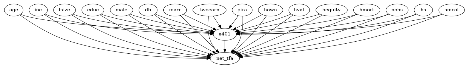
Here we created a simplified graph where there are no interactions between covariates (i.e. nodes in \(X \cup W\)). Most likely, that is not the case in practice. However, as we take joint samples of the covariates—directly from the observed data—later to estimate CATEs, we can ignore their interactions.

Before we assign causal models to variables, let’s plot their histograms to get an idea on the distribution of variables.

import matplotlib.pyplot as plt

cols = [treatment_var, outcome_var]
cols.extend(covariates)
plt.figure(figsize=(10,5))
for i, col in enumerate(cols):
    plt.subplot(3,6,i+1)
    plt.grid(False)
    plt.hist(df[col])
    plt.xlabel(col)
plt.tight_layout()
plt.show()

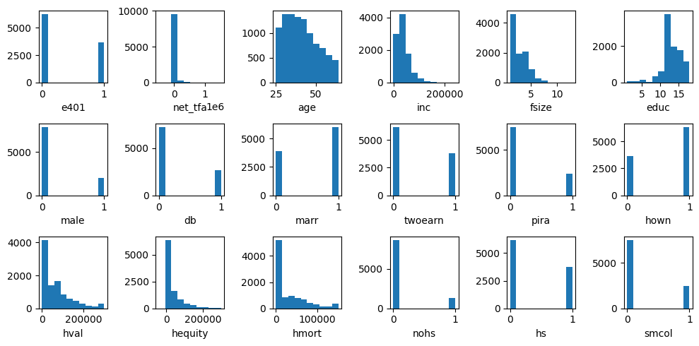
We observe that real-valued variables do not follow well-known parameteric distributions like Gaussian. Therefore, we fit empirical distributions whenever those variables do not have parents, which is also suitable for categorical variables.

Let’s assign causal models to variables. For the treatment variable, we assign a classifier functional causal model (FCM) with a random forest classifier. For the outcome variable, we assign an additive noise model with a random forest regression as a function and empirical distribution for the noise. We assign empirical distributions to other variables as they do not have parents in the causal graph.

causal_model = gcm.StructuralCausalModel(causal_graph)
causal_model.set_causal_mechanism(treatment_var, gcm.ClassifierFCM(gcm.ml.create_random_forest_classifier()))
causal_model.set_causal_mechanism(outcome_var, gcm.AdditiveNoiseModel(gcm.ml.create_random_forest_regressor()))
for covariate in covariates:
    causal_model.set_causal_mechanism(covariate, gcm.EmpiricalDistribution())

To fit a classifier FCM, we cast the treatment column to string type.

df = df.astype({treatment_var: str})

Instead of assigning the models manually, we can also automate this if we don’t have prior knowledge or are not familiar with the statistical implications:

gcm.auto.assign_causal_mechanisms(causal_model, df)

With that, we can now fit the learn the causal models from data.

gcm.fit(causal_model, df)

Fitting causal mechanism of node smcol: 100%|██████████| 18/18 [00:07<00:00,  2.50it/s]

Before computing CATE, we first divide households into equi-width bins of income percentiles. This allows us to study the impact on various income groups.

import numpy as np

percentages = [0.0, 0.2, 0.4, 0.6, 0.8, 1.0]
bin_edges = [0]
bin_edges.extend(np.quantile(df.inc, percentages[1:]).tolist())
bin_edges[-1] += 1 # adding 1 to the last edge as last edge is excluded by np.digitize

groups = [f'{percentages[i]*100:.0f}%-{percentages[i+1]*100:.0f}%' for i in range(len(percentages)-1)]
group_index_to_group_label = dict(zip(range(1, len(bin_edges)+1), groups))

Now we can compute CATE. To this end, we perform a randomised intervention on the treatment variable in the fitted causal graph, draw samples from the interventional distribution, group observations by the income group, and then compute the treatment effect in each group.

np.random.seed(47)

def estimate_cate():
    samples = gcm.interventional_samples(causal_model,
                                         {treatment_var: lambda x: np.random.choice(['0', '1'])},
                                         observed_data=df)
    eligible = samples[treatment_var] == '1'
    ate = samples[eligible][outcome_var].mean() - samples[~eligible][outcome_var].mean()
    result = dict(ate = ate)

    group_indices = np.digitize(samples['inc'], bin_edges)
    samples['group_index'] = group_indices

    for group_index in group_index_to_group_label:
        group_samples = samples[samples['group_index'] == group_index]
        eligible_in_group = group_samples[treatment_var] == '1'
        cate = group_samples[eligible_in_group][outcome_var].mean() - group_samples[~eligible_in_group][outcome_var].mean()
        result[group_index_to_group_label[group_index]] = cate

    return result

group_to_median, group_to_ci = gcm.confidence_intervals(estimate_cate, num_bootstrap_resamples=100)
print(group_to_median)
print(group_to_ci)

Estimating bootstrap interval...: 100%|██████████| 100/100 [01:12<00:00,  1.38it/s]

{'ate': 6531.530932061326, '0%-20%': 3988.627909712817, '20%-40%': 3397.8042844940614, '40%-60%': 5638.570231276086, '60%-80%': 7711.913575250935, '80%-100%': 11712.964337248195}
{'ate': array([4744.72659202, 8481.03233285]), '0%-20%': array([2423.01534603, 5372.78154998]), '20%-40%': array([1422.02052521, 5489.24039284]), '40%-60%': array([3420.0500496 , 8335.78018494]), '60%-80%': array([ 4647.55869618, 11058.51586061]), '80%-100%': array([ 4956.38378325, 18259.26708156])}

The average treatment effect of 401(k) eligibility on net financial assets is positive as indicated by the confidence interval \([4902.24, 8486.89]\). Now, let’s plot CATEs of various income groups to get a clear picture.

fig = plt.figure(figsize=(8,4))
for x, group in enumerate(groups):
    ci = group_to_ci[group]
    plt.plot((x, x), (ci[0], ci[1]), 'ro-', color='orange')
ax = fig.axes[0]
ax.spines['right'].set_visible(False)
ax.spines['top'].set_visible(False)
plt.xticks(range(len(groups)), groups)
plt.xlabel('Income group')
plt.ylabel('ATE of 401(k) eligibility on net financial assets')
plt.show()

/tmp/ipykernel_4672/1344202636.py:4: UserWarning: color is redundantly defined by the 'color' keyword argument and the fmt string "ro-" (-> color='r'). The keyword argument will take precedence.
  plt.plot((x, x), (ci[0], ci[1]), 'ro-', color='orange')

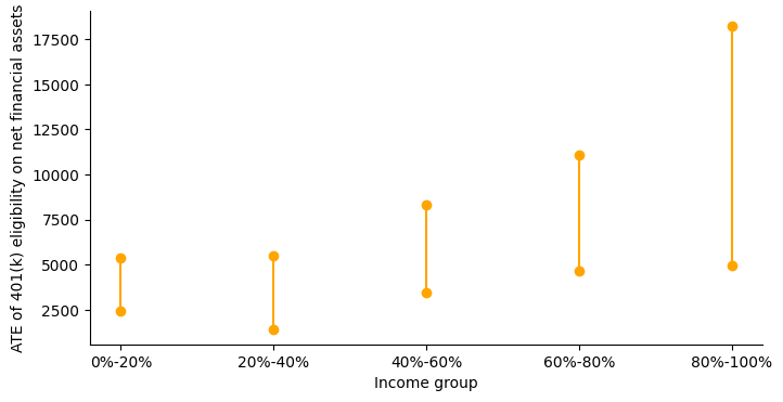
The impact increases as one moves from lower to higher income groups. This result seems to be consistent with the resource constraints of the different income groups.