Estimating effect of multiple treatments
[1]:
import numpy as np
import pandas as pd
import logging

import dowhy
from dowhy import CausalModel
import dowhy.datasets

import econml
import warnings
warnings.filterwarnings('ignore')
[2]:
data = dowhy.datasets.linear_dataset(10, num_common_causes=4, num_samples=10000,
                                    num_instruments=0, num_effect_modifiers=2,
                                     num_treatments=2,
                                    treatment_is_binary=False,
                                    num_discrete_common_causes=2,
                                    num_discrete_effect_modifiers=0,
                                    one_hot_encode=False)
df=data['df']
df.head()
[2]:
| X0 | X1 | W0 | W1 | W2 | W3 | v0 | v1 | y | |
|---|---|---|---|---|---|---|---|---|---|
| 0 | 0.048780 | -1.168705 | 0.542571 | -0.745830 | 0 | 0 | 2.268239 | 3.145854 | 27.554411 |
| 1 | -1.086124 | 1.009211 | -0.788796 | 0.536774 | 2 | 1 | 4.404500 | 7.184804 | 57.884088 |
| 2 | -0.312494 | -0.582138 | 0.519299 | -0.638889 | 0 | 3 | 10.489494 | 1.515061 | 74.968139 |
| 3 | 1.748224 | -0.769179 | 0.278752 | 1.888858 | 3 | 0 | 11.828633 | 18.127881 | 1569.944097 |
| 4 | 0.692610 | 1.158256 | 0.601062 | 0.591958 | 1 | 0 | 6.631769 | 6.379249 | 431.997043 |
[3]:
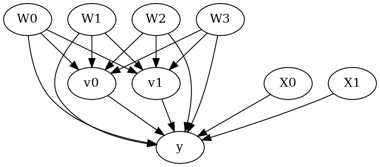
model = CausalModel(data=data["df"],
                    treatment=data["treatment_name"], outcome=data["outcome_name"],
                    graph=data["gml_graph"])
[4]:
model.view_model()
from IPython.display import Image, display
display(Image(filename="causal_model.png"))
[5]:
identified_estimand= model.identify_effect(proceed_when_unidentifiable=True)
print(identified_estimand)
Estimand type: nonparametric-ate

### Estimand : 1
Estimand name: backdoor
Estimand expression:
    d
─────────(E[y|W3,W0,W1,W2])
d[v₀  v₁]
Estimand assumption 1, Unconfoundedness: If U→{v0,v1} and U→y then P(y|v0,v1,W3,W0,W1,W2,U) = P(y|v0,v1,W3,W0,W1,W2)

### Estimand : 2
Estimand name: iv
No such variable(s) found!

### Estimand : 3
Estimand name: frontdoor
No such variable(s) found!
Linear model
Let us first see an example for a linear model. The control_value and treatment_value can be provided as a tuple/list when the treatment is multi-dimensional.
The interpretation is change in y when v0 and v1 are changed from (0,0) to (1,1).
[6]:
linear_estimate = model.estimate_effect(identified_estimand,
                                        method_name="backdoor.linear_regression",
                                       control_value=(0,0),
                                       treatment_value=(1,1),
                                       method_params={'need_conditional_estimates': False})
print(linear_estimate)
*** Causal Estimate ***

## Identified estimand
Estimand type: nonparametric-ate

### Estimand : 1
Estimand name: backdoor
Estimand expression:
    d
─────────(E[y|W3,W0,W1,W2])
d[v₀  v₁]
Estimand assumption 1, Unconfoundedness: If U→{v0,v1} and U→y then P(y|v0,v1,W3,W0,W1,W2,U) = P(y|v0,v1,W3,W0,W1,W2)

## Realized estimand
b: y~v0+v1+W3+W0+W1+W2+v0*X1+v0*X0+v1*X1+v1*X0
Target units: ate

## Estimate
Mean value: 27.598049182644683
You can estimate conditional effects, based on effect modifiers.
[7]:
linear_estimate = model.estimate_effect(identified_estimand,
                                        method_name="backdoor.linear_regression",
                                       control_value=(0,0),
                                       treatment_value=(1,1))
print(linear_estimate)
*** Causal Estimate ***

## Identified estimand
Estimand type: nonparametric-ate

### Estimand : 1
Estimand name: backdoor
Estimand expression:
    d
─────────(E[y|W3,W0,W1,W2])
d[v₀  v₁]
Estimand assumption 1, Unconfoundedness: If U→{v0,v1} and U→y then P(y|v0,v1,W3,W0,W1,W2,U) = P(y|v0,v1,W3,W0,W1,W2)

## Realized estimand
b: y~v0+v1+W3+W0+W1+W2+v0*X1+v0*X0+v1*X1+v1*X0
Target units: ate

## Estimate
Mean value: 27.598049182644683
### Conditional Estimates
__categorical__X1  __categorical__X0
(-4.623, -1.514]   (-3.012, -0.311]    -115.443663
                   (-0.311, 0.273]      -65.270347
                   (0.273, 0.771]       -31.873678
                   (0.771, 1.368]         1.022828
                   (1.368, 5.019]        54.280508
(-1.514, -0.926]   (-3.012, -0.311]     -77.724619
                   (-0.311, 0.273]      -29.198328
                   (0.273, 0.771]         5.232500
                   (0.771, 1.368]        38.251000
                   (1.368, 5.019]        91.802134
(-0.926, -0.416]   (-3.012, -0.311]     -61.536709
                   (-0.311, 0.273]       -5.262257
                   (0.273, 0.771]        27.660328
                   (0.771, 1.368]        61.239789
                   (1.368, 5.019]       114.295588
(-0.416, 0.179]    (-3.012, -0.311]     -39.044539
                   (-0.311, 0.273]       16.329306
                   (0.273, 0.771]        49.838503
                   (0.771, 1.368]        82.778759
                   (1.368, 5.019]       137.403639
(0.179, 3.069]     (-3.012, -0.311]      -1.954634
                   (-0.311, 0.273]       54.155801
                   (0.273, 0.771]        86.890604
                   (0.771, 1.368]       121.662042
                   (1.368, 5.019]       174.116303
dtype: float64
More methods
You can also use methods from EconML or CausalML libraries that support multiple treatments. You can look at examples from the conditional effect notebook: https://py-why.github.io/dowhy/example_notebooks/dowhy-conditional-treatment-effects.html
Propensity-based methods do not support multiple treatments currently.