Conditional Average Treatment Effects (CATE) with DoWhy and EconML
This is an experimental feature where we use EconML methods from DoWhy. Using EconML allows CATE estimation using different methods.
All four steps of causal inference in DoWhy remain the same: model, identify, estimate, and refute. The key difference is that we now call econml methods in the estimation step. There is also a simpler example using linear regression to understand the intuition behind CATE estimators.
All datasets are generated using linear structural equations.
[1]:
%load_ext autoreload
%autoreload 2
[2]:
import numpy as np
import pandas as pd
import logging

import dowhy
from dowhy import CausalModel
import dowhy.datasets

import econml
import warnings
warnings.filterwarnings('ignore')

BETA = 10
[3]:
data = dowhy.datasets.linear_dataset(BETA, num_common_causes=4, num_samples=10000,
                                    num_instruments=2, num_effect_modifiers=2,
                                     num_treatments=1,
                                    treatment_is_binary=False,
                                    num_discrete_common_causes=2,
                                    num_discrete_effect_modifiers=0,
                                    one_hot_encode=False)
df=data['df']
print(df.head())
print("True causal estimate is", data["ate"])
         X0        X1   Z0        Z1        W0        W1 W2 W3         v0  \
0 -1.379763 -1.558929  0.0  0.597805  1.163998  2.189542  2  3  29.315728
1 -1.691229 -1.072651  0.0  0.513919  0.159091  0.785352  1  3  18.817730
2 -0.784829 -2.041068  0.0  0.258637  0.210788  3.549138  1  2  23.105047
3 -0.917294 -1.246345  1.0  0.356331  0.175515  1.657013  1  2  28.248965
4 -1.578481 -0.922904  1.0  0.122975  0.787270  0.753413  3  1  23.992681

            y
0   47.114697
1   68.387037
2   -1.302052
3   94.527411
4  103.142556
True causal estimate is 4.8869819491702104
[4]:
model = CausalModel(data=data["df"],
                    treatment=data["treatment_name"], outcome=data["outcome_name"],
                    graph=data["gml_graph"])
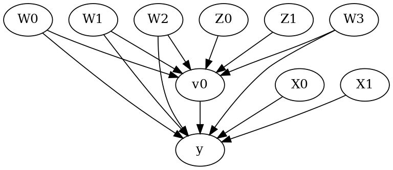
[5]:
model.view_model()
from IPython.display import Image, display
display(Image(filename="causal_model.png"))
[6]:
identified_estimand= model.identify_effect(proceed_when_unidentifiable=True)
print(identified_estimand)
Estimand type: nonparametric-ate

### Estimand : 1
Estimand name: backdoor
Estimand expression:
  d
─────(E[y|W1,W2,W0,W3])
d[v₀]
Estimand assumption 1, Unconfoundedness: If U→{v0} and U→y then P(y|v0,W1,W2,W0,W3,U) = P(y|v0,W1,W2,W0,W3)

### Estimand : 2
Estimand name: iv
Estimand expression:
 ⎡                              -1⎤
 ⎢    d        ⎛    d          ⎞  ⎥
E⎢─────────(y)⋅⎜─────────([v₀])⎟  ⎥
 ⎣d[Z₀  Z₁]    ⎝d[Z₀  Z₁]      ⎠  ⎦
Estimand assumption 1, As-if-random: If U→→y then ¬(U →→{Z0,Z1})
Estimand assumption 2, Exclusion: If we remove {Z0,Z1}→{v0}, then ¬({Z0,Z1}→y)

### Estimand : 3
Estimand name: frontdoor
No such variable(s) found!
Linear Model
First, let us build some intuition using a linear model for estimating CATE. The effect modifiers (that lead to a heterogeneous treatment effect) can be modeled as interaction terms with the treatment. Thus, their value modulates the effect of treatment.
Below the estimated effect of changing treatment from 0 to 1.
[7]:
linear_estimate = model.estimate_effect(identified_estimand,
                                        method_name="backdoor.linear_regression",
                                       control_value=0,
                                       treatment_value=1)
print(linear_estimate)
*** Causal Estimate ***

## Identified estimand
Estimand type: nonparametric-ate

### Estimand : 1
Estimand name: backdoor
Estimand expression:
  d
─────(E[y|W1,W2,W0,W3])
d[v₀]
Estimand assumption 1, Unconfoundedness: If U→{v0} and U→y then P(y|v0,W1,W2,W0,W3,U) = P(y|v0,W1,W2,W0,W3)

## Realized estimand
b: y~v0+W1+W2+W0+W3+v0*X1+v0*X0
Target units: ate

## Estimate
Mean value: 4.887103690062426
### Conditional Estimates
__categorical__X1   __categorical__X0
(-4.673, -1.68]     (-4.557, -1.7]       -3.486745
                    (-1.7, -1.128]       -2.654646
                    (-1.128, -0.628]     -2.102856
                    (-0.628, -0.0255]    -1.441916
                    (-0.0255, 2.929]     -0.714799
(-1.68, -1.107]     (-4.557, -1.7]        0.826901
                    (-1.7, -1.128]        1.698812
                    (-1.128, -0.628]      2.239642
                    (-0.628, -0.0255]     2.780076
                    (-0.0255, 2.929]      3.721243
(-1.107, -0.589]    (-4.557, -1.7]        3.492058
                    (-1.7, -1.128]        4.282674
                    (-1.128, -0.628]      4.888111
                    (-0.628, -0.0255]     5.388771
                    (-0.0255, 2.929]      6.383773
(-0.589, -0.00247]  (-4.557, -1.7]        6.280367
                    (-1.7, -1.128]        7.056493
                    (-1.128, -0.628]      7.517595
                    (-0.628, -0.0255]     8.071627
                    (-0.0255, 2.929]      8.994846
(-0.00247, 2.648]   (-4.557, -1.7]       10.425728
                    (-1.7, -1.128]       11.299806
                    (-1.128, -0.628]     11.763654
                    (-0.628, -0.0255]    12.230149
                    (-0.0255, 2.929]     13.253672
dtype: float64
EconML methods
We now move to the more advanced methods from the EconML package for estimating CATE.
First, let us look at the double machine learning estimator. Method_name corresponds to the fully qualified name of the class that we want to use. For double ML, it is “econml.dml.DML”.
Target units defines the units over which the causal estimate is to be computed. This can be a lambda function filter on the original dataframe, a new Pandas dataframe, or a string corresponding to the three main kinds of target units (“ate”, “att” and “atc”). Below we show an example of a lambda function.
Method_params are passed directly to EconML. For details on allowed parameters, refer to the EconML documentation.
[8]:
from sklearn.preprocessing import PolynomialFeatures
from sklearn.linear_model import LassoCV
from sklearn.ensemble import GradientBoostingRegressor
dml_estimate = model.estimate_effect(identified_estimand, method_name="backdoor.econml.dml.DML",
                                     control_value = 0,
                                     treatment_value = 1,
                                 target_units = lambda df: df["X0"]>1,  # condition used for CATE
                                 confidence_intervals=False,
                                method_params={"init_params":{'model_y':GradientBoostingRegressor(),
                                                              'model_t': GradientBoostingRegressor(),
                                                              "model_final":LassoCV(fit_intercept=False),
                                                              'featurizer':PolynomialFeatures(degree=1, include_bias=False)},
                                               "fit_params":{}})
print(dml_estimate)
2022-09-14 19:14:33.462472: W tensorflow/stream_executor/platform/default/dso_loader.cc:64] Could not load dynamic library 'libcudart.so.11.0'; dlerror: libcudart.so.11.0: cannot open shared object file: No such file or directory
2022-09-14 19:14:33.462513: I tensorflow/stream_executor/cuda/cudart_stub.cc:29] Ignore above cudart dlerror if you do not have a GPU set up on your machine.
*** Causal Estimate ***

## Identified estimand
Estimand type: nonparametric-ate

### Estimand : 1
Estimand name: backdoor
Estimand expression:
  d
─────(E[y|W1,W2,W0,W3])
d[v₀]
Estimand assumption 1, Unconfoundedness: If U→{v0} and U→y then P(y|v0,W1,W2,W0,W3,U) = P(y|v0,W1,W2,W0,W3)

## Realized estimand
b: y~v0+W1+W2+W0+W3 | X1,X0
Target units: Data subset defined by a function

## Estimate
Mean value: 7.249056572837687
Effect estimates: [ 7.63218961 10.67617456 -2.13762711 15.81791602 10.65772066  5.81639516
  4.53340591 17.67893015  0.44013371  9.41423967  9.96734465 15.94945522
 -5.29027534 20.95978919  2.61321796  2.83177785  6.62941359  4.85072387
  8.28435415  3.8783945  12.07111112  3.35030749  2.67247946 14.85530534
  7.32117179 -0.62721827  3.78054571  9.74982175  7.02143449 11.40641448
 -2.82607455 17.99813898  5.93742209 14.77931893  7.98173103 11.99652148
 10.46958908  7.33170987  4.84163327  1.54924715  8.30966962  7.37760578
 10.22868127 14.49903871 14.96352353 12.56389415  5.681735    8.92024655
 -3.91581917 15.96865954  1.17705402 22.43558965 -2.28076389  5.53934221
  0.35869717  7.22578582  7.59419586 19.80896771 12.46234693  7.33632723
  5.71843982 -1.84761763  5.08831316  3.86092668 10.84019564  8.26340317
  4.86542049  5.97761323 16.21383141 11.01651154  5.14148611  5.42555028
  9.20935293 10.32855378  6.77116027  6.83316211  6.37026634 10.55997854
  9.02066328  6.26581433  9.82218573  3.75342187  2.2266487   5.21232068
  5.13491772  8.3604865   9.93320788  3.01404817 -0.28016118  9.21209426
  7.35119211 14.05820121  5.51305571  3.65689354 10.53784127  6.9747079
  1.6505687   7.64252195  3.596969    1.39349191  2.86282336 14.15360907
 11.59044301  1.77017147  1.6197914   6.05462907  3.9359489   6.34571
  3.84761043 15.47922064  7.82213998 13.57697053 10.72942808 13.19086926
  7.14843974 15.19149855 14.44473888  1.86459027  7.24460797  4.1619021
  8.22710628 11.6128131   6.08765849  7.61769251  3.97534736  6.05838589
  5.17106688  5.95267038  5.77435761 11.46540947  6.91723695  6.9259451
 -3.8112268  10.24787725 16.14518099  4.3646474   9.72316641  6.19002146
 -0.91407119  8.32644073  8.88057668  1.19903143  1.76115119  8.2023188
  4.96384976  7.97186163  2.70921309 11.97239826 -2.39964411 11.13296939
  6.85221855  5.99524852 -5.72280421  1.61238488  0.97169628  0.63159157
  0.38906919  1.74640058 14.51077324 -2.21084116  7.93970238  8.23225445
 10.87465176  7.67124388  4.38404006 16.38082756 19.96151678  4.80006542
 10.72805326 12.21879792 13.73603122  6.72726929  8.81285141  0.76258082
 11.62202732  0.24884695 11.35208419  7.47830475 11.2148497   5.57046001
  5.19614461  3.1884282  12.86051641  9.18780449  9.10088187  4.6168349
  5.28096516  6.35288478 12.81778335  7.93465099 10.46238732  8.56093047
  5.92920968  0.31114305  9.54256596  6.27177276 -3.11339008  4.68362665
  6.85653158  5.70137008  0.71747678  7.01668436 10.53492721  3.83863669
  0.31186688  4.57442364  9.17520186  7.90777719  4.3401537   8.26027091
 10.15840794 -1.90645828 11.33959201 16.70585756  3.09530119  7.90676288
  8.27536128  7.36040928 12.73961327  4.21510297  9.71204942  0.57398715
  4.96453601  8.33914499  8.60614054  4.42408661 -0.72206045 10.39402892
  7.39779741  3.91276834 14.77596085  8.04999828 16.00627393  4.54385473
 10.73309693  1.17915851  9.39199326 11.29823627 15.53970036  9.67761757
  9.35214946  7.21085765 11.80624214 12.99830862  8.66237256  9.71009999
  7.94309888  7.83300696  2.26348387 10.52725173  9.60881368  0.40722361
  7.56420975  1.91105729  7.14280047  4.00465455  7.36870956  1.9721601
  8.41457737  3.79455795 12.27095149 16.68539669  4.68308771  6.14076803
 11.20568319  0.68792085 -0.28102034  5.16790436  7.33622205  6.89340439
 -0.48151232  9.47945979 11.31006782  4.81726245  1.36330801 -5.20861339
  1.51898492  4.96439694 17.57613194  9.01010079  6.62616333  3.60269953
  5.08264925  4.86621647 10.77668739  8.88021513  6.92908411  5.34530728
 14.65541517  2.55231055  9.01197395  5.64272237  9.75828995 12.87174451
  5.75557795 -1.3561073  11.6748229   0.6279394   7.9675494   8.8459645
 19.90307618  7.37236094  6.81282222  7.14364384  3.47741632 14.12055391
 15.20943229 15.10779561  3.3113995  17.10199505]
[9]:
print("True causal estimate is", data["ate"])
True causal estimate is 4.8869819491702104
[10]:
dml_estimate = model.estimate_effect(identified_estimand, method_name="backdoor.econml.dml.DML",
                                     control_value = 0,
                                     treatment_value = 1,
                                 target_units = 1,  # condition used for CATE
                                 confidence_intervals=False,
                                method_params={"init_params":{'model_y':GradientBoostingRegressor(),
                                                              'model_t': GradientBoostingRegressor(),
                                                              "model_final":LassoCV(fit_intercept=False),
                                                              'featurizer':PolynomialFeatures(degree=1, include_bias=True)},
                                               "fit_params":{}})
print(dml_estimate)
*** Causal Estimate ***

## Identified estimand
Estimand type: nonparametric-ate

### Estimand : 1
Estimand name: backdoor
Estimand expression:
  d
─────(E[y|W1,W2,W0,W3])
d[v₀]
Estimand assumption 1, Unconfoundedness: If U→{v0} and U→y then P(y|v0,W1,W2,W0,W3,U) = P(y|v0,W1,W2,W0,W3)

## Realized estimand
b: y~v0+W1+W2+W0+W3 | X1,X0
Target units:

## Estimate
Mean value: 4.897085553400156
Effect estimates: [ 0.83779056  2.98311414 -1.00826532 ... -1.1538578  -0.751136
 17.0850596 ]
CATE Object and Confidence Intervals
EconML provides its own methods to compute confidence intervals. Using BootstrapInference in the example below.
[11]:
from sklearn.preprocessing import PolynomialFeatures
from sklearn.linear_model import LassoCV
from sklearn.ensemble import GradientBoostingRegressor
from econml.inference import BootstrapInference
dml_estimate = model.estimate_effect(identified_estimand,
                                     method_name="backdoor.econml.dml.DML",
                                     target_units = "ate",
                                     confidence_intervals=True,
                                     method_params={"init_params":{'model_y':GradientBoostingRegressor(),
                                                              'model_t': GradientBoostingRegressor(),
                                                              "model_final": LassoCV(fit_intercept=False),
                                                              'featurizer':PolynomialFeatures(degree=1, include_bias=True)},
                                               "fit_params":{
                                                               'inference': BootstrapInference(n_bootstrap_samples=100, n_jobs=-1),
                                                            }
                                              })
print(dml_estimate)
*** Causal Estimate ***

## Identified estimand
Estimand type: nonparametric-ate

### Estimand : 1
Estimand name: backdoor
Estimand expression:
  d
─────(E[y|W1,W2,W0,W3])
d[v₀]
Estimand assumption 1, Unconfoundedness: If U→{v0} and U→y then P(y|v0,W1,W2,W0,W3,U) = P(y|v0,W1,W2,W0,W3)

## Realized estimand
b: y~v0+W1+W2+W0+W3 | X1,X0
Target units: ate

## Estimate
Mean value: 4.86715474908683
Effect estimates: [ 0.82092131  2.94307384 -0.99599568 ... -1.1937226  -0.76691448
 17.07340604]
95.0% confidence interval: (array([ 0.68546415,  2.87123464, -1.19802835, ..., -1.47245898,
       -0.982182  , 17.36581825]), array([ 0.813117  ,  2.99322081, -1.01932328, ..., -1.24425797,
       -0.81063881, 17.84794668]))
Can provide a new inputs as target units and estimate CATE on them.
[12]:
test_cols= data['effect_modifier_names'] # only need effect modifiers' values
test_arr = [np.random.uniform(0,1, 10) for _ in range(len(test_cols))] # all variables are sampled uniformly, sample of 10
test_df = pd.DataFrame(np.array(test_arr).transpose(), columns=test_cols)
dml_estimate = model.estimate_effect(identified_estimand,
                                     method_name="backdoor.econml.dml.DML",
                                     target_units = test_df,
                                     confidence_intervals=False,
                                     method_params={"init_params":{'model_y':GradientBoostingRegressor(),
                                                              'model_t': GradientBoostingRegressor(),
                                                              "model_final":LassoCV(),
                                                              'featurizer':PolynomialFeatures(degree=1, include_bias=True)},
                                               "fit_params":{}
                                              })
print(dml_estimate.cate_estimates)
[11.29658774 15.10084253 12.55224943 15.03305186 13.86725959 14.2719788
 13.26797458 14.62508818 12.12506949 14.80787153]
Can also retrieve the raw EconML estimator object for any further operations
[13]:
print(dml_estimate._estimator_object)
<econml.dml.dml.DML object at 0x7fd66efa7a60>
Works with any EconML method
In addition to double machine learning, below we example analyses using orthogonal forests, DRLearner (bug to fix), and neural network-based instrumental variables.
Binary treatment, Binary outcome
[14]:
data_binary = dowhy.datasets.linear_dataset(BETA, num_common_causes=4, num_samples=10000,
                                    num_instruments=2, num_effect_modifiers=2,
                                    treatment_is_binary=True, outcome_is_binary=True)
# convert boolean values to {0,1} numeric
data_binary['df'].v0 = data_binary['df'].v0.astype(int)
data_binary['df'].y = data_binary['df'].y.astype(int)
print(data_binary['df'])

model_binary = CausalModel(data=data_binary["df"],
                    treatment=data_binary["treatment_name"], outcome=data_binary["outcome_name"],
                    graph=data_binary["gml_graph"])
identified_estimand_binary = model_binary.identify_effect(proceed_when_unidentifiable=True)
            X0        X1   Z0        Z1        W0        W1        W2  \
0    -0.676296  2.108027  1.0  0.298524  1.284554 -0.094847  2.163295
1    -0.391211  0.020375  1.0  0.475230  1.134443 -1.008742  1.761336
2     0.172756  1.053240  1.0  0.540688  0.896571  0.438049  0.014401
3     0.819204  0.388839  1.0  0.388804 -1.360003 -1.280483  1.748551
4     0.731195  0.724850  1.0  0.008703 -0.724580 -2.383932  0.207029
...        ...       ...  ...       ...       ...       ...       ...
9995  0.699989 -0.623583  1.0  0.598447  1.619515  0.916936 -1.256653
9996  1.200076  1.338396  1.0  0.853934 -0.640059 -1.176614  2.406046
9997 -0.283139 -0.773638  1.0  0.023027 -1.152597 -0.134382  0.490944
9998 -0.132460  2.373275  1.0  0.977634 -0.525289  2.234319 -0.345546
9999 -0.796017  0.562657  1.0  0.344590 -0.645697  1.091016 -0.531984

            W3  v0  y
0    -1.813771   1  1
1     0.444642   1  1
2    -1.343372   1  1
3     1.824239   1  1
4     1.267825   1  1
...        ...  .. ..
9995  0.034215   1  1
9996 -0.665010   1  1
9997 -0.829003   1  0
9998 -0.244275   1  1
9999  0.115283   1  1

[10000 rows x 10 columns]
Using DRLearner estimator
[15]:
from sklearn.linear_model import LogisticRegressionCV
#todo needs binary y
drlearner_estimate = model_binary.estimate_effect(identified_estimand_binary,
                                method_name="backdoor.econml.drlearner.LinearDRLearner",
                                confidence_intervals=False,
                                method_params={"init_params":{
                                                    'model_propensity': LogisticRegressionCV(cv=3, solver='lbfgs', multi_class='auto')
                                                    },
                                               "fit_params":{}
                                              })
print(drlearner_estimate)
print("True causal estimate is", data_binary["ate"])
*** Causal Estimate ***

## Identified estimand
Estimand type: nonparametric-ate

### Estimand : 1
Estimand name: backdoor
Estimand expression:
  d
─────(E[y|W1,W2,W0,W3])
d[v₀]
Estimand assumption 1, Unconfoundedness: If U→{v0} and U→y then P(y|v0,W1,W2,W0,W3,U) = P(y|v0,W1,W2,W0,W3)

## Realized estimand
b: y~v0+W1+W2+W0+W3 | X1,X0
Target units: ate

## Estimate
Mean value: 0.5617309018550158
Effect estimates: [0.31141911 0.51336777 0.57983555 ... 0.59009221 0.42265299 0.38285284]

True causal estimate is 0.4531
Instrumental Variable Method
[16]:
import keras
from econml.deepiv import DeepIVEstimator
dims_zx = len(model.get_instruments())+len(model.get_effect_modifiers())
dims_tx = len(model._treatment)+len(model.get_effect_modifiers())
treatment_model = keras.Sequential([keras.layers.Dense(128, activation='relu', input_shape=(dims_zx,)), # sum of dims of Z and X
                                    keras.layers.Dropout(0.17),
                                    keras.layers.Dense(64, activation='relu'),
                                    keras.layers.Dropout(0.17),
                                    keras.layers.Dense(32, activation='relu'),
                                    keras.layers.Dropout(0.17)])
response_model = keras.Sequential([keras.layers.Dense(128, activation='relu', input_shape=(dims_tx,)), # sum of dims of T and X
                                    keras.layers.Dropout(0.17),
                                    keras.layers.Dense(64, activation='relu'),
                                    keras.layers.Dropout(0.17),
                                    keras.layers.Dense(32, activation='relu'),
                                    keras.layers.Dropout(0.17),
                                    keras.layers.Dense(1)])

deepiv_estimate = model.estimate_effect(identified_estimand,
                                        method_name="iv.econml.deepiv.DeepIV",
                                        target_units = lambda df: df["X0"]>-1,
                                        confidence_intervals=False,
                                method_params={"init_params":{'n_components': 10, # Number of gaussians in the mixture density networks
                                                              'm': lambda z, x: treatment_model(keras.layers.concatenate([z, x])), # Treatment model,
                                                              "h": lambda t, x: response_model(keras.layers.concatenate([t, x])), # Response model
                                                              'n_samples': 1, # Number of samples used to estimate the response
                                                              'first_stage_options': {'epochs':25},
                                                              'second_stage_options': {'epochs':25}
                                                             },
                                               "fit_params":{}})
print(deepiv_estimate)
2022-09-14 19:17:55.028657: W tensorflow/stream_executor/platform/default/dso_loader.cc:64] Could not load dynamic library 'libcuda.so.1'; dlerror: libcuda.so.1: cannot open shared object file: No such file or directory
2022-09-14 19:17:55.028707: W tensorflow/stream_executor/cuda/cuda_driver.cc:269] failed call to cuInit: UNKNOWN ERROR (303)
2022-09-14 19:17:55.028734: I tensorflow/stream_executor/cuda/cuda_diagnostics.cc:156] kernel driver does not appear to be running on this host (37c5f4ec8b0f): /proc/driver/nvidia/version does not exist
2022-09-14 19:17:55.029027: I tensorflow/core/platform/cpu_feature_guard.cc:193] This TensorFlow binary is optimized with oneAPI Deep Neural Network Library (oneDNN) to use the following CPU instructions in performance-critical operations:  AVX2 AVX512F FMA
To enable them in other operations, rebuild TensorFlow with the appropriate compiler flags.
Epoch 1/25
313/313 [==============================] - 1s 2ms/step - loss: 9.3995
Epoch 2/25
313/313 [==============================] - 1s 2ms/step - loss: 3.4535
Epoch 3/25
313/313 [==============================] - 1s 2ms/step - loss: 2.7533
Epoch 4/25
313/313 [==============================] - 1s 2ms/step - loss: 2.6117
Epoch 5/25
313/313 [==============================] - 1s 2ms/step - loss: 2.5759
Epoch 6/25
313/313 [==============================] - 1s 2ms/step - loss: 2.5326
Epoch 7/25
313/313 [==============================] - 1s 2ms/step - loss: 2.5116
Epoch 8/25
313/313 [==============================] - 1s 2ms/step - loss: 2.4777
Epoch 9/25
313/313 [==============================] - 1s 2ms/step - loss: 2.4666
Epoch 10/25
313/313 [==============================] - 1s 2ms/step - loss: 2.4424
Epoch 11/25
313/313 [==============================] - 1s 2ms/step - loss: 2.4419
Epoch 12/25
313/313 [==============================] - 1s 2ms/step - loss: 2.4274
Epoch 13/25
313/313 [==============================] - 1s 2ms/step - loss: 2.4194
Epoch 14/25
313/313 [==============================] - 1s 2ms/step - loss: 2.4108
Epoch 15/25
313/313 [==============================] - 1s 2ms/step - loss: 2.4025
Epoch 16/25
313/313 [==============================] - 1s 2ms/step - loss: 2.3893
Epoch 17/25
313/313 [==============================] - 1s 2ms/step - loss: 2.3965
Epoch 18/25
313/313 [==============================] - 1s 2ms/step - loss: 2.3810
Epoch 19/25
313/313 [==============================] - 1s 2ms/step - loss: 2.3607
Epoch 20/25
313/313 [==============================] - 1s 2ms/step - loss: 2.3590
Epoch 21/25
313/313 [==============================] - 1s 2ms/step - loss: 2.3537
Epoch 22/25
313/313 [==============================] - 1s 2ms/step - loss: 2.3461
Epoch 23/25
313/313 [==============================] - 1s 2ms/step - loss: 2.3459
Epoch 24/25
313/313 [==============================] - 1s 2ms/step - loss: 2.3375
Epoch 25/25
313/313 [==============================] - 1s 2ms/step - loss: 2.3350
Epoch 1/25
313/313 [==============================] - 2s 2ms/step - loss: 10536.4648
Epoch 2/25
313/313 [==============================] - 1s 2ms/step - loss: 6305.3052
Epoch 3/25
313/313 [==============================] - 1s 2ms/step - loss: 4151.0879
Epoch 4/25
313/313 [==============================] - 1s 2ms/step - loss: 3740.7751
Epoch 5/25
313/313 [==============================] - 1s 2ms/step - loss: 3738.5132
Epoch 6/25
313/313 [==============================] - 1s 2ms/step - loss: 3629.3538
Epoch 7/25
313/313 [==============================] - 1s 2ms/step - loss: 3583.9417
Epoch 8/25
313/313 [==============================] - 1s 2ms/step - loss: 3505.2583
Epoch 9/25
313/313 [==============================] - 1s 2ms/step - loss: 3555.1487
Epoch 10/25
313/313 [==============================] - 1s 2ms/step - loss: 3522.9038
Epoch 11/25
313/313 [==============================] - 1s 2ms/step - loss: 3508.9656
Epoch 12/25
313/313 [==============================] - 1s 2ms/step - loss: 3513.9800
Epoch 13/25
313/313 [==============================] - 1s 2ms/step - loss: 3443.2627
Epoch 14/25
313/313 [==============================] - 1s 2ms/step - loss: 3442.2480
Epoch 15/25
313/313 [==============================] - 1s 2ms/step - loss: 3393.5464
Epoch 16/25
313/313 [==============================] - 1s 2ms/step - loss: 3502.4641
Epoch 17/25
313/313 [==============================] - 1s 2ms/step - loss: 3431.1438
Epoch 18/25
313/313 [==============================] - 1s 3ms/step - loss: 3283.8574
Epoch 19/25
313/313 [==============================] - 1s 2ms/step - loss: 3447.3086
Epoch 20/25
313/313 [==============================] - 1s 2ms/step - loss: 3481.0642
Epoch 21/25
313/313 [==============================] - 1s 2ms/step - loss: 3391.8186
Epoch 22/25
313/313 [==============================] - 1s 2ms/step - loss: 3448.9109
Epoch 23/25
313/313 [==============================] - 1s 2ms/step - loss: 3432.2117
Epoch 24/25
313/313 [==============================] - 1s 2ms/step - loss: 3498.3252
Epoch 25/25
313/313 [==============================] - 1s 2ms/step - loss: 3469.0784
WARNING:tensorflow:
The following Variables were used a Lambda layer's call (lambda_7), but
are not present in its tracked objects:
  <tf.Variable 'dense_3/kernel:0' shape=(3, 128) dtype=float32>
  <tf.Variable 'dense_3/bias:0' shape=(128,) dtype=float32>
  <tf.Variable 'dense_4/kernel:0' shape=(128, 64) dtype=float32>
  <tf.Variable 'dense_4/bias:0' shape=(64,) dtype=float32>
  <tf.Variable 'dense_5/kernel:0' shape=(64, 32) dtype=float32>
  <tf.Variable 'dense_5/bias:0' shape=(32,) dtype=float32>
  <tf.Variable 'dense_6/kernel:0' shape=(32, 1) dtype=float32>
  <tf.Variable 'dense_6/bias:0' shape=(1,) dtype=float32>
It is possible that this is intended behavior, but it is more likely
an omission. This is a strong indication that this layer should be
formulated as a subclassed Layer rather than a Lambda layer.
173/173 [==============================] - 0s 1ms/step
173/173 [==============================] - 0s 1ms/step
*** Causal Estimate ***

## Identified estimand
Estimand type: nonparametric-ate

### Estimand : 1
Estimand name: iv
Estimand expression:
 ⎡                              -1⎤
 ⎢    d        ⎛    d          ⎞  ⎥
E⎢─────────(y)⋅⎜─────────([v₀])⎟  ⎥
 ⎣d[Z₀  Z₁]    ⎝d[Z₀  Z₁]      ⎠  ⎦
Estimand assumption 1, As-if-random: If U→→y then ¬(U →→{Z0,Z1})
Estimand assumption 2, Exclusion: If we remove {Z0,Z1}→{v0}, then ¬({Z0,Z1}→y)

## Realized estimand
b: y~v0+W1+W2+W0+W3 | X1,X0
Target units: Data subset defined by a function

## Estimate
Mean value: 0.6664953231811523
Effect estimates: [-0.48396087  0.8478241   2.4622421  ... -0.3602295  -0.00521469
  2.8501587 ]
Metalearners
[17]:
data_experiment = dowhy.datasets.linear_dataset(BETA, num_common_causes=5, num_samples=10000,
                                    num_instruments=2, num_effect_modifiers=5,
                                    treatment_is_binary=True, outcome_is_binary=False)
# convert boolean values to {0,1} numeric
data_experiment['df'].v0 = data_experiment['df'].v0.astype(int)
print(data_experiment['df'])
model_experiment = CausalModel(data=data_experiment["df"],
                    treatment=data_experiment["treatment_name"], outcome=data_experiment["outcome_name"],
                    graph=data_experiment["gml_graph"])
identified_estimand_experiment = model_experiment.identify_effect(proceed_when_unidentifiable=True)
            X0        X1        X2        X3        X4   Z0        Z1  \
0     0.450545 -1.257515  0.471642 -1.470290 -0.313567  0.0  0.725650
1    -1.203378 -1.157465  1.382549 -0.583257  2.169368  1.0  0.794024
2    -0.594827 -0.915781 -0.239883 -1.932128  1.746734  1.0  0.879416
3     0.111767 -0.218169  1.033464 -0.789402  0.969954  0.0  0.416110
4     1.204116  0.198154  1.049902 -1.062127  0.917942  1.0  0.554945
...        ...       ...       ...       ...       ...  ...       ...
9995 -0.574383  0.614512  0.415807 -1.657983  0.992253  1.0  0.663603
9996 -0.183360  1.652605  1.197322 -1.799480  0.601277  0.0  0.601031
9997 -0.289223 -0.717008  0.778591  0.426638  0.884653  1.0  0.703789
9998 -0.187420 -0.086943 -0.134770 -1.095107  1.812915  1.0  0.333952
9999  0.261882 -2.917083  0.478326 -1.436661  3.546299  1.0  0.773814

            W0        W1        W2        W3        W4  v0          y
0    -0.472835 -0.997446  0.004614  0.017763  0.478225   1   0.556320
1    -0.515159 -1.079848 -0.245822 -1.584561  0.234426   1  -0.491323
2     1.291060  0.626573 -0.090517 -0.314269 -0.327587   1   2.004246
3     1.149823 -1.106448 -1.527173 -0.596446  0.055568   0  -7.201138
4    -0.015453 -1.462126 -1.198382 -0.784080  0.537499   1   7.922537
...        ...       ...       ...       ...       ...  ..        ...
9995  0.389882  0.509070  0.201076 -1.215764  0.640585   1   2.940028
9996 -1.848232 -0.046541 -1.764638 -1.929402  1.117040   0  -8.504087
9997 -2.148089 -0.390873 -1.502542 -1.204583  0.096626   1   5.443509
9998  1.003753  0.651637  0.006543 -1.325260  0.990296   1   9.078075
9999  0.791542 -2.691675 -0.760971 -2.787962  0.818148   0 -21.582046

[10000 rows x 14 columns]
[18]:
from sklearn.ensemble import RandomForestRegressor
metalearner_estimate = model_experiment.estimate_effect(identified_estimand_experiment,
                                method_name="backdoor.econml.metalearners.TLearner",
                                confidence_intervals=False,
                                method_params={"init_params":{
                                                    'models': RandomForestRegressor()
                                                    },
                                               "fit_params":{}
                                              })
print(metalearner_estimate)
print("True causal estimate is", data_experiment["ate"])
*** Causal Estimate ***

## Identified estimand
Estimand type: nonparametric-ate

### Estimand : 1
Estimand name: backdoor
Estimand expression:
  d
─────(E[y|W1,W2,W0,W4,W3])
d[v₀]
Estimand assumption 1, Unconfoundedness: If U→{v0} and U→y then P(y|v0,W1,W2,W0,W4,W3,U) = P(y|v0,W1,W2,W0,W4,W3)

## Realized estimand
b: y~v0+X4+X3+X1+X0+X2+W1+W2+W0+W4+W3
Target units: ate

## Estimate
Mean value: 12.170173158123257
Effect estimates: [ 4.28288619 11.05004512  5.2743599  ... 13.76848574 11.52333009
 19.04514471]

True causal estimate is 9.232266234493785
Avoiding retraining the estimator
Once an estimator is fitted, it can be reused to estimate effect on different data points. In this case, you can pass fit_estimator=False to estimate_effect. This works for any EconML estimator. We show an example for the T-learner below.
[19]:
# For metalearners, need to provide all the features (except treatmeant and outcome)
metalearner_estimate = model_experiment.estimate_effect(identified_estimand_experiment,
                                method_name="backdoor.econml.metalearners.TLearner",
                                confidence_intervals=False,
                                fit_estimator=False,
                                target_units=data_experiment["df"].drop(["v0","y", "Z0", "Z1"], axis=1)[9995:],
                                method_params={})
print(metalearner_estimate)
print("True causal estimate is", data_experiment["ate"])
*** Causal Estimate ***

## Identified estimand
Estimand type: nonparametric-ate

### Estimand : 1
Estimand name: backdoor
Estimand expression:
  d
─────(E[y|W1,W2,W0,W4,W3])
d[v₀]
Estimand assumption 1, Unconfoundedness: If U→{v0} and U→y then P(y|v0,W1,W2,W0,W4,W3,U) = P(y|v0,W1,W2,W0,W4,W3)

## Realized estimand
b: y~v0+X4+X3+X1+X0+X2+W1+W2+W0+W4+W3
Target units: Data subset provided as a data frame

## Estimate
Mean value: 14.007555135107586
Effect estimates: [16.19153226 18.60039497 13.37967147 15.34281126  6.52336571]

True causal estimate is 9.232266234493785
Refuting the estimate
Adding a random common cause variable
[20]:
res_random=model.refute_estimate(identified_estimand, dml_estimate, method_name="random_common_cause")
print(res_random)
Refute: Add a random common cause
Estimated effect:13.69479737527619
New effect:13.683336990621342
p value:0.8200000000000001
Adding an unobserved common cause variable
[21]:
res_unobserved=model.refute_estimate(identified_estimand, dml_estimate, method_name="add_unobserved_common_cause",
                                     confounders_effect_on_treatment="linear", confounders_effect_on_outcome="linear",
                                    effect_strength_on_treatment=0.01, effect_strength_on_outcome=0.02)
print(res_unobserved)
Refute: Add an Unobserved Common Cause
Estimated effect:13.69479737527619
New effect:13.692495592526896
Replacing treatment with a random (placebo) variable
[22]:
res_placebo=model.refute_estimate(identified_estimand, dml_estimate,
        method_name="placebo_treatment_refuter", placebo_type="permute",
        num_simulations=10 # at least 100 is good, setting to 10 for speed
        )
print(res_placebo)
Refute: Use a Placebo Treatment
Estimated effect:13.69479737527619
New effect:0.016450445501047732
p value:0.3932817279521587
Removing a random subset of the data
[23]:
res_subset=model.refute_estimate(identified_estimand, dml_estimate,
        method_name="data_subset_refuter", subset_fraction=0.8,
        num_simulations=10)
print(res_subset)
Refute: Use a subset of data
Estimated effect:13.69479737527619
New effect:13.72601340772405
p value:0.3080393048064634
More refutation methods to come, especially specific to the CATE estimators.