DoWhy: Different estimation methods for causal inference

This is a quick introduction to the DoWhy causal inference library. We will load in a sample dataset and use different methods for estimating the causal effect of a (pre-specified)treatment variable on a (pre-specified) outcome variable.

We will see that not all estimators return the correct effect for this dataset.

First, let us add the required path for Python to find the DoWhy code and load all required packages

[1]:

%load_ext autoreload
%autoreload 2

[2]:

import numpy as np
import pandas as pd
import logging

import dowhy
from dowhy import CausalModel
import dowhy.datasets

Now, let us load a dataset. For simplicity, we simulate a dataset with linear relationships between common causes and treatment, and common causes and outcome.

Beta is the true causal effect.

[3]:

data = dowhy.datasets.linear_dataset(beta=10,
        num_common_causes=5,
        num_instruments = 2,
        num_treatments=1,
        num_samples=10000,
        treatment_is_binary=True,
        outcome_is_binary=False,
        stddev_treatment_noise=10)
df = data["df"]
df

[3]:

	Z0	Z1	W0	W1	W2	W3	W4	v0	y
0	1.0	0.687986	1.633494	-1.250625	0.927178	-1.833909	-0.404578	True	5.498197
1	1.0	0.756570	0.398974	-1.389788	1.146683	-2.245861	-0.845968	True	1.782328
2	1.0	0.875724	-1.170325	-0.138730	2.203882	-0.030699	-1.603035	True	4.628401
3	0.0	0.924126	-0.951097	0.675440	0.480698	-0.861801	-2.738749	False	-12.592867
4	0.0	0.605515	-0.342407	1.448468	1.408716	-2.028318	-0.414919	True	13.333022
...	...	...	...	...	...	...	...	...	...
9995	0.0	0.056583	-0.011412	-3.570399	1.246381	-0.298294	-2.293432	False	-21.295866
9996	1.0	0.504050	-0.747385	-0.053360	0.117537	-1.425899	-1.864726	False	-11.462042
9997	1.0	0.904261	0.228929	-1.418597	0.218014	-0.802668	-0.169217	True	4.449252
9998	1.0	0.380770	-0.407239	0.672763	2.566541	-2.290793	0.009718	True	15.038049
9999	1.0	0.141680	-0.730638	0.052157	0.420813	-1.127148	-0.508346	True	6.775777

10000 rows × 9 columns

Note that we are using a pandas dataframe to load the data.

Identifying the causal estimand

We now input a causal graph in the DOT graph format.

[4]:

# With graph
model=CausalModel(
        data = df,
        treatment=data["treatment_name"],
        outcome=data["outcome_name"],
        graph=data["gml_graph"],
        instruments=data["instrument_names"]
        )

[5]:

model.view_model()

[6]:

from IPython.display import Image, display
display(Image(filename="causal_model.png"))

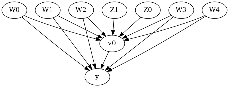
../_images/example_notebooks_dowhy_estimation_methods_10_0.png

We get a causal graph. Now identification and estimation is done.

[7]:

identified_estimand = model.identify_effect(proceed_when_unidentifiable=True)
print(identified_estimand)

Estimand type: nonparametric-ate

### Estimand : 1
Estimand name: backdoor
Estimand expression:
  d
─────(E[y|W4,W3,W0,W1,W2])
d[v₀]
Estimand assumption 1, Unconfoundedness: If U→{v0} and U→y then P(y|v0,W4,W3,W0,W1,W2,U) = P(y|v0,W4,W3,W0,W1,W2)

### Estimand : 2
Estimand name: iv
Estimand expression:
 ⎡                              -1⎤
 ⎢    d        ⎛    d          ⎞  ⎥
E⎢─────────(y)⋅⎜─────────([v₀])⎟  ⎥
 ⎣d[Z₁  Z₀]    ⎝d[Z₁  Z₀]      ⎠  ⎦
Estimand assumption 1, As-if-random: If U→→y then ¬(U →→{Z1,Z0})
Estimand assumption 2, Exclusion: If we remove {Z1,Z0}→{v0}, then ¬({Z1,Z0}→y)

### Estimand : 3
Estimand name: frontdoor
No such variable(s) found!

Method 1: Regression

Use linear regression.

[8]:

causal_estimate_reg = model.estimate_effect(identified_estimand,
        method_name="backdoor.linear_regression",
        test_significance=True)
print(causal_estimate_reg)
print("Causal Estimate is " + str(causal_estimate_reg.value))

*** Causal Estimate ***

## Identified estimand
Estimand type: nonparametric-ate

### Estimand : 1
Estimand name: backdoor
Estimand expression:
  d
─────(E[y|W4,W3,W0,W1,W2])
d[v₀]
Estimand assumption 1, Unconfoundedness: If U→{v0} and U→y then P(y|v0,W4,W3,W0,W1,W2,U) = P(y|v0,W4,W3,W0,W1,W2)

## Realized estimand
b: y~v0+W4+W3+W0+W1+W2
Target units: ate

## Estimate
Mean value: 10.00004796011746
p-value: [0.]

Causal Estimate is 10.00004796011746

Method 2: Distance Matching

Define a distance metric and then use the metric to match closest points between treatment and control.

[9]:

causal_estimate_dmatch = model.estimate_effect(identified_estimand,
                                              method_name="backdoor.distance_matching",
                                              target_units="att",
                                              method_params={'distance_metric':"minkowski", 'p':2})
print(causal_estimate_dmatch)
print("Causal Estimate is " + str(causal_estimate_dmatch.value))

*** Causal Estimate ***

## Identified estimand
Estimand type: nonparametric-ate

### Estimand : 1
Estimand name: backdoor
Estimand expression:
  d
─────(E[y|W4,W3,W0,W1,W2])
d[v₀]
Estimand assumption 1, Unconfoundedness: If U→{v0} and U→y then P(y|v0,W4,W3,W0,W1,W2,U) = P(y|v0,W4,W3,W0,W1,W2)

## Realized estimand
b: y~v0+W4+W3+W0+W1+W2
Target units: att

## Estimate
Mean value: 10.500365546485488

Causal Estimate is 10.500365546485488

Method 3: Propensity Score Stratification

We will be using propensity scores to stratify units in the data.

[10]:

causal_estimate_strat = model.estimate_effect(identified_estimand,
                                              method_name="backdoor.propensity_score_stratification",
                                              target_units="att")
print(causal_estimate_strat)
print("Causal Estimate is " + str(causal_estimate_strat.value))

*** Causal Estimate ***

## Identified estimand
Estimand type: nonparametric-ate

### Estimand : 1
Estimand name: backdoor
Estimand expression:
  d
─────(E[y|W4,W3,W0,W1,W2])
d[v₀]
Estimand assumption 1, Unconfoundedness: If U→{v0} and U→y then P(y|v0,W4,W3,W0,W1,W2,U) = P(y|v0,W4,W3,W0,W1,W2)

## Realized estimand
b: y~v0+W4+W3+W0+W1+W2
Target units: att

## Estimate
Mean value: 10.091725925183123

Causal Estimate is 10.091725925183123

Method 4: Propensity Score Matching

We will be using propensity scores to match units in the data.

[11]:

causal_estimate_match = model.estimate_effect(identified_estimand,
                                              method_name="backdoor.propensity_score_matching",
                                              target_units="atc")
print(causal_estimate_match)
print("Causal Estimate is " + str(causal_estimate_match.value))

*** Causal Estimate ***

## Identified estimand
Estimand type: nonparametric-ate

### Estimand : 1
Estimand name: backdoor
Estimand expression:
  d
─────(E[y|W4,W3,W0,W1,W2])
d[v₀]
Estimand assumption 1, Unconfoundedness: If U→{v0} and U→y then P(y|v0,W4,W3,W0,W1,W2,U) = P(y|v0,W4,W3,W0,W1,W2)

## Realized estimand
b: y~v0+W4+W3+W0+W1+W2
Target units: atc

## Estimate
Mean value: 9.850957370560343

Causal Estimate is 9.850957370560343

Method 5: Weighting

We will be using (inverse) propensity scores to assign weights to units in the data. DoWhy supports a few different weighting schemes: 1. Vanilla Inverse Propensity Score weighting (IPS) (weighting_scheme=“ips_weight”) 2. Self-normalized IPS weighting (also known as the Hajek estimator) (weighting_scheme=“ips_normalized_weight”) 3. Stabilized IPS weighting (weighting_scheme = “ips_stabilized_weight”)

[12]:

causal_estimate_ipw = model.estimate_effect(identified_estimand,
                                            method_name="backdoor.propensity_score_weighting",
                                            target_units = "ate",
                                            method_params={"weighting_scheme":"ips_weight"})
print(causal_estimate_ipw)
print("Causal Estimate is " + str(causal_estimate_ipw.value))

*** Causal Estimate ***

## Identified estimand
Estimand type: nonparametric-ate

### Estimand : 1
Estimand name: backdoor
Estimand expression:
  d
─────(E[y|W4,W3,W0,W1,W2])
d[v₀]
Estimand assumption 1, Unconfoundedness: If U→{v0} and U→y then P(y|v0,W4,W3,W0,W1,W2,U) = P(y|v0,W4,W3,W0,W1,W2)

## Realized estimand
b: y~v0+W4+W3+W0+W1+W2
Target units: ate

## Estimate
Mean value: 10.184880436277249

Causal Estimate is 10.184880436277249

Method 6: Instrumental Variable

We will be using the Wald estimator for the provided instrumental variable.

[13]:

causal_estimate_iv = model.estimate_effect(identified_estimand,
        method_name="iv.instrumental_variable", method_params = {'iv_instrument_name': 'Z0'})
print(causal_estimate_iv)
print("Causal Estimate is " + str(causal_estimate_iv.value))

*** Causal Estimate ***

## Identified estimand
Estimand type: nonparametric-ate

### Estimand : 1
Estimand name: iv
Estimand expression:
 ⎡                              -1⎤
 ⎢    d        ⎛    d          ⎞  ⎥
E⎢─────────(y)⋅⎜─────────([v₀])⎟  ⎥
 ⎣d[Z₁  Z₀]    ⎝d[Z₁  Z₀]      ⎠  ⎦
Estimand assumption 1, As-if-random: If U→→y then ¬(U →→{Z1,Z0})
Estimand assumption 2, Exclusion: If we remove {Z1,Z0}→{v0}, then ¬({Z1,Z0}→y)

## Realized estimand
Realized estimand: Wald Estimator
Realized estimand type: nonparametric-ate
Estimand expression:
 ⎡ d    ⎤  -1⎡ d     ⎤
E⎢───(y)⎥⋅E  ⎢───(v₀)⎥
 ⎣dZ₀   ⎦    ⎣dZ₀    ⎦
Estimand assumption 1, As-if-random: If U→→y then ¬(U →→{Z1,Z0})
Estimand assumption 2, Exclusion: If we remove {Z1,Z0}→{v0}, then ¬({Z1,Z0}→y)
Estimand assumption 3, treatment_effect_homogeneity: Each unit's treatment ['v0'] is affected in the same way by common causes of ['v0'] and y
Estimand assumption 4, outcome_effect_homogeneity: Each unit's outcome y is affected in the same way by common causes of ['v0'] and y

Target units: ate

## Estimate
Mean value: 10.253272548814012

Causal Estimate is 10.253272548814012

Method 7: Regression Discontinuity

We will be internally converting this to an equivalent instrumental variables problem.

[14]:

causal_estimate_regdist = model.estimate_effect(identified_estimand,
        method_name="iv.regression_discontinuity",
        method_params={'rd_variable_name':'Z1',
                       'rd_threshold_value':0.5,
                       'rd_bandwidth': 0.15})
print(causal_estimate_regdist)
print("Causal Estimate is " + str(causal_estimate_regdist.value))

*** Causal Estimate ***

## Identified estimand
Estimand type: nonparametric-ate

### Estimand : 1
Estimand name: iv
Estimand expression:
 ⎡                              -1⎤
 ⎢    d        ⎛    d          ⎞  ⎥
E⎢─────────(y)⋅⎜─────────([v₀])⎟  ⎥
 ⎣d[Z₁  Z₀]    ⎝d[Z₁  Z₀]      ⎠  ⎦
Estimand assumption 1, As-if-random: If U→→y then ¬(U →→{Z1,Z0})
Estimand assumption 2, Exclusion: If we remove {Z1,Z0}→{v0}, then ¬({Z1,Z0}→y)

## Realized estimand
Realized estimand: Wald Estimator
Realized estimand type: nonparametric-ate
Estimand expression:
 ⎡        d            ⎤  -1⎡        d             ⎤
E⎢──────────────────(y)⎥⋅E  ⎢──────────────────(v₀)⎥
 ⎣dlocal_rd_variable   ⎦    ⎣dlocal_rd_variable    ⎦
Estimand assumption 1, As-if-random: If U→→y then ¬(U →→{Z1,Z0})
Estimand assumption 2, Exclusion: If we remove {Z1,Z0}→{v0}, then ¬({Z1,Z0}→y)
Estimand assumption 3, treatment_effect_homogeneity: Each unit's treatment ['local_treatment'] is affected in the same way by common causes of ['local_treatment'] and local_outcome
Estimand assumption 4, outcome_effect_homogeneity: Each unit's outcome local_outcome is affected in the same way by common causes of ['local_treatment'] and local_outcome

Target units: ate

## Estimate
Mean value: -1.3421212407734997

Causal Estimate is -1.3421212407734997