Demo for the DoWhy causal API

We show a simple example of adding a causal extension to any dataframe.

import dowhy.datasets
import dowhy.api

import numpy as np
import pandas as pd

from statsmodels.api import OLS

data = dowhy.datasets.linear_dataset(beta=5,
        num_common_causes=1,
        num_instruments = 0,
        num_samples=1000,
        treatment_is_binary=True)
df = data['df']
df['y'] = df['y'] + np.random.normal(size=len(df)) # Adding noise to data. Without noise, the variance in Y|X, Z is zero, and mcmc fails.
#data['dot_graph'] = 'digraph { v ->y;X0-> v;X0-> y;}'

treatment= data["treatment_name"][0]
outcome = data["outcome_name"][0]
common_cause = data["common_causes_names"][0]
df

	W0	v0	y
0	0.339059	False	1.523297
1	1.009676	True	4.361143
2	0.376290	True	7.623149
3	0.832195	True	6.504141
4	0.585708	True	4.155991
...	...	...	...
995	-0.560865	False	-2.036794
996	-0.439966	False	-1.173392
997	-1.545073	False	-2.369035
998	1.565063	True	5.896693
999	-1.197883	True	2.477574

1000 rows × 3 columns

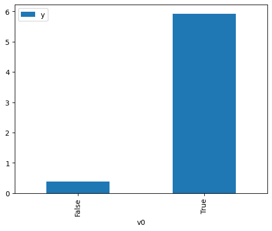
# data['df'] is just a regular pandas.DataFrame
df.causal.do(x=treatment,
                     variable_types={treatment: 'b', outcome: 'c', common_cause: 'c'},
                     outcome=outcome,
                     common_causes=[common_cause],
                     proceed_when_unidentifiable=True).groupby(treatment).mean().plot(y=outcome, kind='bar')

<AxesSubplot:xlabel='v0'>

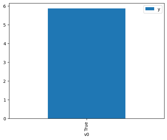
df.causal.do(x={treatment: 1},
              variable_types={treatment:'b', outcome: 'c', common_cause: 'c'},
              outcome=outcome,
              method='weighting',
              common_causes=[common_cause],
              proceed_when_unidentifiable=True).groupby(treatment).mean().plot(y=outcome, kind='bar')

<AxesSubplot:xlabel='v0'>

cdf_1 = df.causal.do(x={treatment: 1},
              variable_types={treatment: 'b', outcome: 'c', common_cause: 'c'},
              outcome=outcome,
              dot_graph=data['dot_graph'],
              proceed_when_unidentifiable=True)

cdf_0 = df.causal.do(x={treatment: 0},
              variable_types={treatment: 'b', outcome: 'c', common_cause: 'c'},
              outcome=outcome,
              dot_graph=data['dot_graph'],
              proceed_when_unidentifiable=True)

cdf_0

	W0	v0	y	propensity_score	weight
0	-0.370839	False	-1.426270	0.668533	1.495812
1	1.956810	False	1.876996	0.017484	57.195309
2	-0.382916	False	-1.248201	0.673950	1.483791
3	0.924422	False	1.606464	0.126667	7.894687
4	0.789872	False	1.731581	0.160123	6.245181
...	...	...	...	...	...
995	1.518796	False	2.492069	0.041540	24.073284
996	1.617724	False	3.848876	0.034233	29.211278
997	1.956810	False	1.876996	0.017484	57.195309
998	-0.185325	False	-0.376236	0.580432	1.722855
999	0.177932	False	0.086486	0.398028	2.512383

1000 rows × 5 columns

cdf_1

	W0	v0	y	propensity_score	weight
0	-0.592847	True	3.291838	0.239989	4.166851
1	1.404890	True	4.027509	0.948201	1.054629
2	0.727954	True	5.849403	0.822222	1.216216
3	-0.582116	True	4.759021	0.243990	4.098536
4	-0.085492	True	4.919241	0.469623	2.129369
...	...	...	...	...	...
995	0.064974	True	4.467355	0.545902	1.831831
996	0.821375	True	3.852592	0.848300	1.178828
997	1.791186	True	6.668863	0.975690	1.024916
998	-0.507771	True	3.795654	0.272923	3.664033
999	0.393533	True	5.167014	0.700954	1.426627

1000 rows × 5 columns

Comparing the estimate to Linear Regression

First, estimating the effect using the causal data frame, and the 95% confidence interval.

(cdf_1['y'] - cdf_0['y']).mean()

$\displaystyle 5.39681422096609$

1.96*(cdf_1['y'] - cdf_0['y']).std() / np.sqrt(len(df))

$\displaystyle 0.134680784526509$

Comparing to the estimate from OLS.

model = OLS(np.asarray(df[outcome]), np.asarray(df[[common_cause, treatment]], dtype=np.float64))
result = model.fit()
result.summary()

OLS Regression Results

Dep. Variable:	y	R-squared (uncentered):	0.966
Model:	OLS	Adj. R-squared (uncentered):	0.966
Method:	Least Squares	F-statistic:	1.407e+04
Date:	Wed, 14 Sep 2022	Prob (F-statistic):	0.00
Time:	19:25:36	Log-Likelihood:	-1439.7
No. Observations:	1000	AIC:	2883.
Df Residuals:	998	BIC:	2893.
Df Model:	2
Covariance Type:	nonrobust

	coef	std err	t	P>|t|	[0.025	0.975]
x1	1.2791	0.039	32.390	0.000	1.202	1.357
x2	5.0288	0.056	89.202	0.000	4.918	5.139

Omnibus:	3.317	Durbin-Watson:	1.975
Prob(Omnibus):	0.190	Jarque-Bera (JB):	3.386
Skew:	0.130	Prob(JB):	0.184
Kurtosis:	2.884	Cond. No.	2.74

Notes:
[1] R² is computed without centering (uncentered) since the model does not contain a constant.
[2] Standard Errors assume that the covariance matrix of the errors is correctly specified.