Estimating effect of multiple treatments
[1]:
import numpy as np
import pandas as pd
import logging

import dowhy
from dowhy import CausalModel
import dowhy.datasets

import econml
import warnings
warnings.filterwarnings('ignore')
[2]:
data = dowhy.datasets.linear_dataset(10, num_common_causes=4, num_samples=10000,
                                    num_instruments=0, num_effect_modifiers=2,
                                     num_treatments=2,
                                    treatment_is_binary=False,
                                    num_discrete_common_causes=2,
                                    num_discrete_effect_modifiers=0,
                                    one_hot_encode=False)
df=data['df']
df.head()
[2]:
| X0 | X1 | W0 | W1 | W2 | W3 | v0 | v1 | y | |
|---|---|---|---|---|---|---|---|---|---|
| 0 | -0.614298 | -1.186804 | -1.224096 | -2.465764 | 0 | 0 | -11.985166 | -3.117210 | -365.334500 |
| 1 | -1.815659 | -0.593030 | -0.942089 | -1.978565 | 3 | 0 | -3.185456 | 10.173167 | 408.634756 |
| 2 | 0.149613 | -1.995628 | -0.247485 | -1.167555 | 1 | 0 | -0.777541 | 2.817673 | 24.801607 |
| 3 | -0.608667 | -1.211001 | 1.019357 | -0.172742 | 1 | 3 | 12.525051 | 20.015384 | -1002.628091 |
| 4 | -0.070603 | -2.974622 | 0.061755 | 0.799555 | 1 | 1 | 8.808388 | 8.910479 | -265.978142 |
[3]:
model = CausalModel(data=data["df"],
                    treatment=data["treatment_name"], outcome=data["outcome_name"],
                    graph=data["gml_graph"])
[4]:
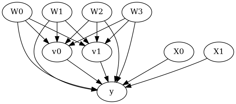
model.view_model()
from IPython.display import Image, display
display(Image(filename="causal_model.png"))
[5]:
identified_estimand= model.identify_effect(proceed_when_unidentifiable=True)
print(identified_estimand)
Estimand type: nonparametric-ate

### Estimand : 1
Estimand name: backdoor
Estimand expression:
    d
─────────(E[y|W1,W0,W2,W3])
d[v₀  v₁]
Estimand assumption 1, Unconfoundedness: If U→{v0,v1} and U→y then P(y|v0,v1,W1,W0,W2,W3,U) = P(y|v0,v1,W1,W0,W2,W3)

### Estimand : 2
Estimand name: iv
No such variable(s) found!

### Estimand : 3
Estimand name: frontdoor
No such variable(s) found!
Linear model
Let us first see an example for a linear model. The control_value and treatment_value can be provided as a tuple/list when the treatment is multi-dimensional.
The interpretation is change in y when v0 and v1 are changed from (0,0) to (1,1).
[6]:
linear_estimate = model.estimate_effect(identified_estimand,
                                        method_name="backdoor.linear_regression",
                                       control_value=(0,0),
                                       treatment_value=(1,1),
                                       method_params={'need_conditional_estimates': False})
print(linear_estimate)
*** Causal Estimate ***

## Identified estimand
Estimand type: nonparametric-ate

### Estimand : 1
Estimand name: backdoor
Estimand expression:
    d
─────────(E[y|W1,W0,W2,W3])
d[v₀  v₁]
Estimand assumption 1, Unconfoundedness: If U→{v0,v1} and U→y then P(y|v0,v1,W1,W0,W2,W3,U) = P(y|v0,v1,W1,W0,W2,W3)

## Realized estimand
b: y~v0+v1+W1+W0+W2+W3+v0*X1+v0*X0+v1*X1+v1*X0
Target units: ate

## Estimate
Mean value: -66.74442465406742
You can estimate conditional effects, based on effect modifiers.
[7]:
linear_estimate = model.estimate_effect(identified_estimand,
                                        method_name="backdoor.linear_regression",
                                       control_value=(0,0),
                                       treatment_value=(1,1))
print(linear_estimate)
*** Causal Estimate ***

## Identified estimand
Estimand type: nonparametric-ate

### Estimand : 1
Estimand name: backdoor
Estimand expression:
    d
─────────(E[y|W1,W0,W2,W3])
d[v₀  v₁]
Estimand assumption 1, Unconfoundedness: If U→{v0,v1} and U→y then P(y|v0,v1,W1,W0,W2,W3,U) = P(y|v0,v1,W1,W0,W2,W3)

## Realized estimand
b: y~v0+v1+W1+W0+W2+W3+v0*X1+v0*X0+v1*X1+v1*X0
Target units: ate

## Estimate
Mean value: -66.74442465406742
### Conditional Estimates
__categorical__X1  __categorical__X0
(-4.729, -1.777]   (-4.679, -1.53]     -220.871781
                   (-1.53, -0.956]     -150.155692
                   (-0.956, -0.447]    -109.691028
                   (-0.447, 0.133]      -65.408004
                   (0.133, 3.604]         2.041486
(-1.777, -1.193]   (-4.679, -1.53]     -189.994985
                   (-1.53, -0.956]     -123.059891
                   (-0.956, -0.447]     -81.895146
                   (-0.447, 0.133]      -40.701964
                   (0.133, 3.604]        27.022741
(-1.193, -0.7]     (-4.679, -1.53]     -175.043669
                   (-1.53, -0.956]     -107.080577
                   (-0.956, -0.447]     -66.362576
                   (-0.447, 0.133]      -24.914318
                   (0.133, 3.604]        41.026608
(-0.7, -0.0978]    (-4.679, -1.53]     -159.866871
                   (-1.53, -0.956]      -93.306996
                   (-0.956, -0.447]     -50.013717
                   (-0.447, 0.133]      -10.095979
                   (0.133, 3.604]        56.802998
(-0.0978, 3.745]   (-4.679, -1.53]     -135.286454
                   (-1.53, -0.956]      -64.496616
                   (-0.956, -0.447]     -24.495949
                   (-0.447, 0.133]       14.385220
                   (0.133, 3.604]        82.289652
dtype: float64
More methods
You can also use methods from EconML or CausalML libraries that support multiple treatments. You can look at examples from the conditional effect notebook: https://microsoft.github.io/dowhy/example_notebooks/dowhy-conditional-treatment-effects.html
Propensity-based methods do not support multiple treatments currently.