Conditional Average Treatment Effects (CATE) with DoWhy and EconML
This is an experimental feature where we use EconML methods from DoWhy. Using EconML allows CATE estimation using different methods.
All four steps of causal inference in DoWhy remain the same: model, identify, estimate, and refute. The key difference is that we now call econml methods in the estimation step. There is also a simpler example using linear regression to understand the intuition behind CATE estimators.
All datasets are generated using linear structural equations.
[1]:
%load_ext autoreload
%autoreload 2
[2]:
import numpy as np
import pandas as pd
import logging

import dowhy
from dowhy import CausalModel
import dowhy.datasets

import econml
import warnings
warnings.filterwarnings('ignore')

BETA = 10
[3]:
data = dowhy.datasets.linear_dataset(BETA, num_common_causes=4, num_samples=10000,
                                    num_instruments=2, num_effect_modifiers=2,
                                     num_treatments=1,
                                    treatment_is_binary=False,
                                    num_discrete_common_causes=2,
                                    num_discrete_effect_modifiers=0,
                                    one_hot_encode=False)
df=data['df']
print(df.head())
print("True causal estimate is", data["ate"])
         X0        X1   Z0        Z1        W0        W1 W2 W3         v0  \
0 -0.533201 -1.022194  0.0  0.179820 -0.126268 -0.665279  0  2   0.377309
1  1.922557 -0.762009  0.0  0.899564 -0.229440 -1.197794  1  1   9.944403
2  1.171414  1.479419  1.0  0.513904  0.987447  0.439091  0  2  24.655594
3  0.484425 -1.845972  0.0  0.387353  1.517763 -0.685227  0  3  13.782830
4  1.122992  0.385469  0.0  0.313835  0.115356  2.225336  1  1  17.397334

            y
0    1.888306
1   84.051100
2  399.830888
3   65.517166
4  220.655496
True causal estimate is 9.049694403977
[4]:
model = CausalModel(data=data["df"],
                    treatment=data["treatment_name"], outcome=data["outcome_name"],
                    graph=data["gml_graph"])
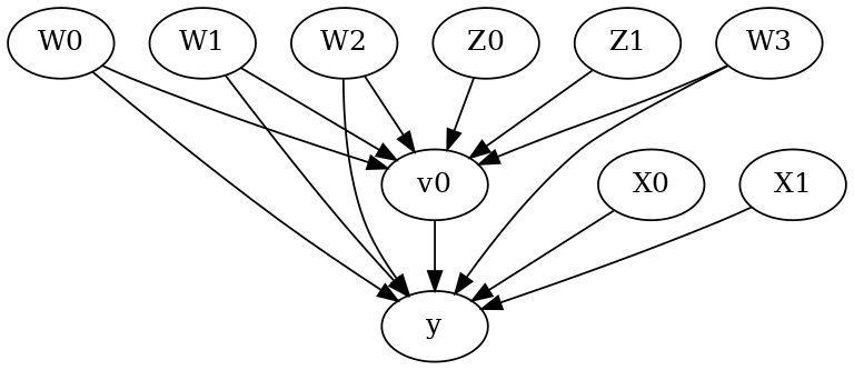
[5]:
model.view_model()
from IPython.display import Image, display
display(Image(filename="causal_model.png"))
[6]:
identified_estimand= model.identify_effect(proceed_when_unidentifiable=True)
print(identified_estimand)
Estimand type: nonparametric-ate

### Estimand : 1
Estimand name: backdoor
Estimand expression:
  d
─────(E[y|W2,W0,W1,W3])
d[v₀]
Estimand assumption 1, Unconfoundedness: If U→{v0} and U→y then P(y|v0,W2,W0,W1,W3,U) = P(y|v0,W2,W0,W1,W3)

### Estimand : 2
Estimand name: iv
Estimand expression:
 ⎡                              -1⎤
 ⎢    d        ⎛    d          ⎞  ⎥
E⎢─────────(y)⋅⎜─────────([v₀])⎟  ⎥
 ⎣d[Z₀  Z₁]    ⎝d[Z₀  Z₁]      ⎠  ⎦
Estimand assumption 1, As-if-random: If U→→y then ¬(U →→{Z0,Z1})
Estimand assumption 2, Exclusion: If we remove {Z0,Z1}→{v0}, then ¬({Z0,Z1}→y)

### Estimand : 3
Estimand name: frontdoor
No such variable(s) found!
Linear Model
First, let us build some intuition using a linear model for estimating CATE. The effect modifiers (that lead to a heterogeneous treatment effect) can be modeled as interaction terms with the treatment. Thus, their value modulates the effect of treatment.
Below the estimated effect of changing treatment from 0 to 1.
[7]:
linear_estimate = model.estimate_effect(identified_estimand,
                                        method_name="backdoor.linear_regression",
                                       control_value=0,
                                       treatment_value=1)
print(linear_estimate)
*** Causal Estimate ***

## Identified estimand
Estimand type: nonparametric-ate

### Estimand : 1
Estimand name: backdoor
Estimand expression:
  d
─────(E[y|W2,W0,W1,W3])
d[v₀]
Estimand assumption 1, Unconfoundedness: If U→{v0} and U→y then P(y|v0,W2,W0,W1,W3,U) = P(y|v0,W2,W0,W1,W3)

## Realized estimand
b: y~v0+W2+W0+W1+W3+v0*X0+v0*X1
Target units: ate

## Estimate
Mean value: 9.049415183121157
### Conditional Estimates
__categorical__X0              __categorical__X1
(-3.5749999999999997, -0.687]  (-4.484, -1.15]       3.288129
                               (-1.15, -0.562]       6.267303
                               (-0.562, -0.0573]     8.040084
                               (-0.0573, 0.538]      9.904973
                               (0.538, 3.207]       12.728653
(-0.687, -0.0947]              (-4.484, -1.15]       3.897843
                               (-1.15, -0.562]       6.885845
                               (-0.562, -0.0573]     8.702318
                               (-0.0573, 0.538]     10.441822
                               (0.538, 3.207]       13.349133
(-0.0947, 0.407]               (-4.484, -1.15]       4.452250
                               (-1.15, -0.562]       7.266740
                               (-0.562, -0.0573]     9.058710
                               (-0.0573, 0.538]     10.834069
                               (0.538, 3.207]       13.682690
(0.407, 0.987]                 (-4.484, -1.15]       4.755422
                               (-1.15, -0.562]       7.603704
                               (-0.562, -0.0573]     9.435272
                               (-0.0573, 0.538]     11.217643
                               (0.538, 3.207]       14.214437
(0.987, 4.197]                 (-4.484, -1.15]       5.298979
                               (-1.15, -0.562]       8.278518
                               (-0.562, -0.0573]    10.018361
                               (-0.0573, 0.538]     11.803522
                               (0.538, 3.207]       14.808277
dtype: float64
EconML methods
We now move to the more advanced methods from the EconML package for estimating CATE.
First, let us look at the double machine learning estimator. Method_name corresponds to the fully qualified name of the class that we want to use. For double ML, it is “econml.dml.DML”.
Target units defines the units over which the causal estimate is to be computed. This can be a lambda function filter on the original dataframe, a new Pandas dataframe, or a string corresponding to the three main kinds of target units (“ate”, “att” and “atc”). Below we show an example of a lambda function.
Method_params are passed directly to EconML. For details on allowed parameters, refer to the EconML documentation.
[8]:
from sklearn.preprocessing import PolynomialFeatures
from sklearn.linear_model import LassoCV
from sklearn.ensemble import GradientBoostingRegressor
dml_estimate = model.estimate_effect(identified_estimand, method_name="backdoor.econml.dml.DML",
                                     control_value = 0,
                                     treatment_value = 1,
                                 target_units = lambda df: df["X0"]>1,  # condition used for CATE
                                 confidence_intervals=False,
                                method_params={"init_params":{'model_y':GradientBoostingRegressor(),
                                                              'model_t': GradientBoostingRegressor(),
                                                              "model_final":LassoCV(fit_intercept=False),
                                                              'featurizer':PolynomialFeatures(degree=1, include_bias=False)},
                                               "fit_params":{}})
print(dml_estimate)
2022-09-14 18:44:20.050299: W tensorflow/stream_executor/platform/default/dso_loader.cc:64] Could not load dynamic library 'libcudart.so.11.0'; dlerror: libcudart.so.11.0: cannot open shared object file: No such file or directory
2022-09-14 18:44:20.050337: I tensorflow/stream_executor/cuda/cudart_stub.cc:29] Ignore above cudart dlerror if you do not have a GPU set up on your machine.
*** Causal Estimate ***

## Identified estimand
Estimand type: nonparametric-ate

### Estimand : 1
Estimand name: backdoor
Estimand expression:
  d
─────(E[y|W2,W0,W1,W3])
d[v₀]
Estimand assumption 1, Unconfoundedness: If U→{v0} and U→y then P(y|v0,W2,W0,W1,W3,U) = P(y|v0,W2,W0,W1,W3)

## Realized estimand
b: y~v0+W2+W0+W1+W3 | X0,X1
Target units: Data subset defined by a function

## Estimate
Mean value: 10.073101008999998
Effect estimates: [ 8.75174232 15.87229533 12.10883134 ...  7.61828507  2.48628422
  9.32302822]
[9]:
print("True causal estimate is", data["ate"])
True causal estimate is 9.049694403977
[10]:
dml_estimate = model.estimate_effect(identified_estimand, method_name="backdoor.econml.dml.DML",
                                     control_value = 0,
                                     treatment_value = 1,
                                 target_units = 1,  # condition used for CATE
                                 confidence_intervals=False,
                                method_params={"init_params":{'model_y':GradientBoostingRegressor(),
                                                              'model_t': GradientBoostingRegressor(),
                                                              "model_final":LassoCV(fit_intercept=False),
                                                              'featurizer':PolynomialFeatures(degree=1, include_bias=True)},
                                               "fit_params":{}})
print(dml_estimate)
*** Causal Estimate ***

## Identified estimand
Estimand type: nonparametric-ate

### Estimand : 1
Estimand name: backdoor
Estimand expression:
  d
─────(E[y|W2,W0,W1,W3])
d[v₀]
Estimand assumption 1, Unconfoundedness: If U→{v0} and U→y then P(y|v0,W2,W0,W1,W3,U) = P(y|v0,W2,W0,W1,W3)

## Realized estimand
b: y~v0+W2+W0+W1+W3 | X0,X1
Target units:

## Estimate
Mean value: 9.0105851188843
Effect estimates: [ 6.15557119  8.64699923 15.73603354 ... 15.87179788  8.05935455
  8.75923011]
CATE Object and Confidence Intervals
EconML provides its own methods to compute confidence intervals. Using BootstrapInference in the example below.
[11]:
from sklearn.preprocessing import PolynomialFeatures
from sklearn.linear_model import LassoCV
from sklearn.ensemble import GradientBoostingRegressor
from econml.inference import BootstrapInference
dml_estimate = model.estimate_effect(identified_estimand,
                                     method_name="backdoor.econml.dml.DML",
                                     target_units = "ate",
                                     confidence_intervals=True,
                                     method_params={"init_params":{'model_y':GradientBoostingRegressor(),
                                                              'model_t': GradientBoostingRegressor(),
                                                              "model_final": LassoCV(fit_intercept=False),
                                                              'featurizer':PolynomialFeatures(degree=1, include_bias=True)},
                                               "fit_params":{
                                                               'inference': BootstrapInference(n_bootstrap_samples=100, n_jobs=-1),
                                                            }
                                              })
print(dml_estimate)
*** Causal Estimate ***

## Identified estimand
Estimand type: nonparametric-ate

### Estimand : 1
Estimand name: backdoor
Estimand expression:
  d
─────(E[y|W2,W0,W1,W3])
d[v₀]
Estimand assumption 1, Unconfoundedness: If U→{v0} and U→y then P(y|v0,W2,W0,W1,W3,U) = P(y|v0,W2,W0,W1,W3)

## Realized estimand
b: y~v0+W2+W0+W1+W3 | X0,X1
Target units: ate

## Estimate
Mean value: 8.97103120997889
Effect estimates: [ 6.11637397  8.57762811 15.70466462 ... 15.84544308  8.00633323
  8.73332712]
95.0% confidence interval: (array([ 6.04294108,  8.42758643, 15.77291365, ..., 15.92144005,
        7.93937896,  8.75143052]), array([ 6.18996505,  8.66689443, 16.17018427, ..., 16.33172413,
        8.06900788,  8.91158551]))
Can provide a new inputs as target units and estimate CATE on them.
[12]:
test_cols= data['effect_modifier_names'] # only need effect modifiers' values
test_arr = [np.random.uniform(0,1, 10) for _ in range(len(test_cols))] # all variables are sampled uniformly, sample of 10
test_df = pd.DataFrame(np.array(test_arr).transpose(), columns=test_cols)
dml_estimate = model.estimate_effect(identified_estimand,
                                     method_name="backdoor.econml.dml.DML",
                                     target_units = test_df,
                                     confidence_intervals=False,
                                     method_params={"init_params":{'model_y':GradientBoostingRegressor(),
                                                              'model_t': GradientBoostingRegressor(),
                                                              "model_final":LassoCV(),
                                                              'featurizer':PolynomialFeatures(degree=1, include_bias=True)},
                                               "fit_params":{}
                                              })
print(dml_estimate.cate_estimates)
[11.04119185 13.14994662 10.35837984 12.47894912 11.36113085 13.39935511
 13.90418027 10.28889381 12.38958317 12.97335591]
Can also retrieve the raw EconML estimator object for any further operations
[13]:
print(dml_estimate._estimator_object)
<econml.dml.dml.DML object at 0x7f0cf55373a0>
Works with any EconML method
In addition to double machine learning, below we example analyses using orthogonal forests, DRLearner (bug to fix), and neural network-based instrumental variables.
Binary treatment, Binary outcome
[14]:
data_binary = dowhy.datasets.linear_dataset(BETA, num_common_causes=4, num_samples=10000,
                                    num_instruments=2, num_effect_modifiers=2,
                                    treatment_is_binary=True, outcome_is_binary=True)
# convert boolean values to {0,1} numeric
data_binary['df'].v0 = data_binary['df'].v0.astype(int)
data_binary['df'].y = data_binary['df'].y.astype(int)
print(data_binary['df'])

model_binary = CausalModel(data=data_binary["df"],
                    treatment=data_binary["treatment_name"], outcome=data_binary["outcome_name"],
                    graph=data_binary["gml_graph"])
identified_estimand_binary = model_binary.identify_effect(proceed_when_unidentifiable=True)
            X0        X1   Z0        Z1        W0        W1        W2  \
0    -0.977022  1.067383  1.0  0.696816  0.877629 -0.704097 -2.705619
1     0.119435  1.646813  1.0  0.932599  1.045068 -1.503361 -0.811373
2     2.368885  2.055748  1.0  0.551497  0.832655 -0.056771 -2.144246
3    -0.256994  0.945261  1.0  0.614187 -1.904988 -1.624514 -1.838845
4     2.329471  1.215418  1.0  0.647074  2.402067 -0.312094 -1.590205
...        ...       ...  ...       ...       ...       ...       ...
9995  1.327564  3.895272  0.0  0.974441  1.724229 -0.534615  0.062941
9996  0.095342  1.142415  1.0  0.890541  1.315665 -0.436278 -0.964123
9997  0.909117  1.771237  1.0  0.402906  1.189027 -0.175096 -0.514647
9998  0.199285  2.383161  1.0  0.166742 -1.331729 -0.409680 -0.525951
9999  2.682434  0.140926  1.0  0.880121  0.744858 -0.319757 -1.370824

            W3  v0  y
0    -1.050106   1  1
1    -0.392080   1  1
2    -1.936656   1  1
3     0.332871   1  1
4    -0.294840   1  1
...        ...  .. ..
9995 -1.546670   1  1
9996  0.571672   1  1
9997 -1.751814   1  1
9998 -0.603038   1  1
9999 -0.995968   1  1

[10000 rows x 10 columns]
Using DRLearner estimator
[15]:
from sklearn.linear_model import LogisticRegressionCV
#todo needs binary y
drlearner_estimate = model_binary.estimate_effect(identified_estimand_binary,
                                method_name="backdoor.econml.drlearner.LinearDRLearner",
                                confidence_intervals=False,
                                method_params={"init_params":{
                                                    'model_propensity': LogisticRegressionCV(cv=3, solver='lbfgs', multi_class='auto')
                                                    },
                                               "fit_params":{}
                                              })
print(drlearner_estimate)
print("True causal estimate is", data_binary["ate"])
*** Causal Estimate ***

## Identified estimand
Estimand type: nonparametric-ate

### Estimand : 1
Estimand name: backdoor
Estimand expression:
  d
─────(E[y|W2,W0,W1,W3])
d[v₀]
Estimand assumption 1, Unconfoundedness: If U→{v0} and U→y then P(y|v0,W2,W0,W1,W3,U) = P(y|v0,W2,W0,W1,W3)

## Realized estimand
b: y~v0+W2+W0+W1+W3 | X0,X1
Target units: ate

## Estimate
Mean value: 0.6073356972078376
Effect estimates: [0.64530812 0.64334411 0.61774472 ... 0.633828   0.66240192 0.55963395]

True causal estimate is 0.4818
Instrumental Variable Method
[16]:
import keras
from econml.deepiv import DeepIVEstimator
dims_zx = len(model.get_instruments())+len(model.get_effect_modifiers())
dims_tx = len(model._treatment)+len(model.get_effect_modifiers())
treatment_model = keras.Sequential([keras.layers.Dense(128, activation='relu', input_shape=(dims_zx,)), # sum of dims of Z and X
                                    keras.layers.Dropout(0.17),
                                    keras.layers.Dense(64, activation='relu'),
                                    keras.layers.Dropout(0.17),
                                    keras.layers.Dense(32, activation='relu'),
                                    keras.layers.Dropout(0.17)])
response_model = keras.Sequential([keras.layers.Dense(128, activation='relu', input_shape=(dims_tx,)), # sum of dims of T and X
                                    keras.layers.Dropout(0.17),
                                    keras.layers.Dense(64, activation='relu'),
                                    keras.layers.Dropout(0.17),
                                    keras.layers.Dense(32, activation='relu'),
                                    keras.layers.Dropout(0.17),
                                    keras.layers.Dense(1)])

deepiv_estimate = model.estimate_effect(identified_estimand,
                                        method_name="iv.econml.deepiv.DeepIV",
                                        target_units = lambda df: df["X0"]>-1,
                                        confidence_intervals=False,
                                method_params={"init_params":{'n_components': 10, # Number of gaussians in the mixture density networks
                                                              'm': lambda z, x: treatment_model(keras.layers.concatenate([z, x])), # Treatment model,
                                                              "h": lambda t, x: response_model(keras.layers.concatenate([t, x])), # Response model
                                                              'n_samples': 1, # Number of samples used to estimate the response
                                                              'first_stage_options': {'epochs':25},
                                                              'second_stage_options': {'epochs':25}
                                                             },
                                               "fit_params":{}})
print(deepiv_estimate)
2022-09-14 18:47:39.639288: W tensorflow/stream_executor/platform/default/dso_loader.cc:64] Could not load dynamic library 'libcuda.so.1'; dlerror: libcuda.so.1: cannot open shared object file: No such file or directory
2022-09-14 18:47:39.639334: W tensorflow/stream_executor/cuda/cuda_driver.cc:269] failed call to cuInit: UNKNOWN ERROR (303)
2022-09-14 18:47:39.639362: I tensorflow/stream_executor/cuda/cuda_diagnostics.cc:156] kernel driver does not appear to be running on this host (37c5f4ec8b0f): /proc/driver/nvidia/version does not exist
2022-09-14 18:47:39.639675: I tensorflow/core/platform/cpu_feature_guard.cc:193] This TensorFlow binary is optimized with oneAPI Deep Neural Network Library (oneDNN) to use the following CPU instructions in performance-critical operations:  AVX2 AVX512F FMA
To enable them in other operations, rebuild TensorFlow with the appropriate compiler flags.
Epoch 1/25
313/313 [==============================] - 1s 2ms/step - loss: 11.9591
Epoch 2/25
313/313 [==============================] - 1s 2ms/step - loss: 4.0460
Epoch 3/25
313/313 [==============================] - 1s 2ms/step - loss: 3.3135
Epoch 4/25
313/313 [==============================] - 1s 2ms/step - loss: 2.7917
Epoch 5/25
313/313 [==============================] - 1s 2ms/step - loss: 2.6947
Epoch 6/25
313/313 [==============================] - 1s 2ms/step - loss: 2.6366
Epoch 7/25
313/313 [==============================] - 1s 2ms/step - loss: 2.6077
Epoch 8/25
313/313 [==============================] - 1s 2ms/step - loss: 2.5855
Epoch 9/25
313/313 [==============================] - 1s 2ms/step - loss: 2.5629
Epoch 10/25
313/313 [==============================] - 1s 2ms/step - loss: 2.5409
Epoch 11/25
313/313 [==============================] - 1s 2ms/step - loss: 2.5363
Epoch 12/25
313/313 [==============================] - 1s 2ms/step - loss: 2.5217
Epoch 13/25
313/313 [==============================] - 1s 2ms/step - loss: 2.5183
Epoch 14/25
313/313 [==============================] - 1s 2ms/step - loss: 2.5099
Epoch 15/25
313/313 [==============================] - 1s 2ms/step - loss: 2.5105
Epoch 16/25
313/313 [==============================] - 1s 2ms/step - loss: 2.5087
Epoch 17/25
313/313 [==============================] - 1s 2ms/step - loss: 2.4881
Epoch 18/25
313/313 [==============================] - 1s 2ms/step - loss: 2.4904
Epoch 19/25
313/313 [==============================] - 1s 2ms/step - loss: 2.4946
Epoch 20/25
313/313 [==============================] - 1s 2ms/step - loss: 2.4887
Epoch 21/25
313/313 [==============================] - 1s 2ms/step - loss: 2.4925
Epoch 22/25
313/313 [==============================] - 1s 2ms/step - loss: 2.4871
Epoch 23/25
313/313 [==============================] - 1s 2ms/step - loss: 2.4811
Epoch 24/25
313/313 [==============================] - 1s 2ms/step - loss: 2.4775
Epoch 25/25
313/313 [==============================] - 1s 2ms/step - loss: 2.4735
Epoch 1/25
313/313 [==============================] - 2s 2ms/step - loss: 21077.2461
Epoch 2/25
313/313 [==============================] - 1s 2ms/step - loss: 10133.7412
Epoch 3/25
313/313 [==============================] - 1s 2ms/step - loss: 8876.9043
Epoch 4/25
313/313 [==============================] - 1s 2ms/step - loss: 8798.7510
Epoch 5/25
313/313 [==============================] - 1s 2ms/step - loss: 8595.7393
Epoch 6/25
313/313 [==============================] - 1s 2ms/step - loss: 8717.2373
Epoch 7/25
313/313 [==============================] - 1s 2ms/step - loss: 8639.3955
Epoch 8/25
313/313 [==============================] - 1s 2ms/step - loss: 8385.5654
Epoch 9/25
313/313 [==============================] - 1s 2ms/step - loss: 8489.7207
Epoch 10/25
313/313 [==============================] - 1s 2ms/step - loss: 8431.2227
Epoch 11/25
313/313 [==============================] - 1s 2ms/step - loss: 8506.2080
Epoch 12/25
313/313 [==============================] - 1s 2ms/step - loss: 8443.2041
Epoch 13/25
313/313 [==============================] - 1s 2ms/step - loss: 8480.6875
Epoch 14/25
313/313 [==============================] - 1s 2ms/step - loss: 8212.8369
Epoch 15/25
313/313 [==============================] - 1s 2ms/step - loss: 8410.5000
Epoch 16/25
313/313 [==============================] - 1s 2ms/step - loss: 8186.9043
Epoch 17/25
313/313 [==============================] - 1s 2ms/step - loss: 8367.1201
Epoch 18/25
313/313 [==============================] - 1s 2ms/step - loss: 8283.7197
Epoch 19/25
313/313 [==============================] - 1s 2ms/step - loss: 8472.3135
Epoch 20/25
313/313 [==============================] - 1s 2ms/step - loss: 8411.8926
Epoch 21/25
313/313 [==============================] - 1s 2ms/step - loss: 8463.8564
Epoch 22/25
313/313 [==============================] - 1s 2ms/step - loss: 8485.9541
Epoch 23/25
313/313 [==============================] - 1s 2ms/step - loss: 8202.4541
Epoch 24/25
313/313 [==============================] - 1s 3ms/step - loss: 8426.0312
Epoch 25/25
313/313 [==============================] - 1s 2ms/step - loss: 8251.6318
WARNING:tensorflow:
The following Variables were used a Lambda layer's call (lambda_7), but
are not present in its tracked objects:
  <tf.Variable 'dense_3/kernel:0' shape=(3, 128) dtype=float32>
  <tf.Variable 'dense_3/bias:0' shape=(128,) dtype=float32>
  <tf.Variable 'dense_4/kernel:0' shape=(128, 64) dtype=float32>
  <tf.Variable 'dense_4/bias:0' shape=(64,) dtype=float32>
  <tf.Variable 'dense_5/kernel:0' shape=(64, 32) dtype=float32>
  <tf.Variable 'dense_5/bias:0' shape=(32,) dtype=float32>
  <tf.Variable 'dense_6/kernel:0' shape=(32, 1) dtype=float32>
  <tf.Variable 'dense_6/bias:0' shape=(1,) dtype=float32>
It is possible that this is intended behavior, but it is more likely
an omission. This is a strong indication that this layer should be
formulated as a subclassed Layer rather than a Lambda layer.
273/273 [==============================] - 0s 969us/step
273/273 [==============================] - 0s 989us/step
*** Causal Estimate ***

## Identified estimand
Estimand type: nonparametric-ate

### Estimand : 1
Estimand name: iv
Estimand expression:
 ⎡                              -1⎤
 ⎢    d        ⎛    d          ⎞  ⎥
E⎢─────────(y)⋅⎜─────────([v₀])⎟  ⎥
 ⎣d[Z₀  Z₁]    ⎝d[Z₀  Z₁]      ⎠  ⎦
Estimand assumption 1, As-if-random: If U→→y then ¬(U →→{Z0,Z1})
Estimand assumption 2, Exclusion: If we remove {Z0,Z1}→{v0}, then ¬({Z0,Z1}→y)

## Realized estimand
b: y~v0+W2+W0+W1+W3 | X0,X1
Target units: Data subset defined by a function

## Estimate
Mean value: -0.0007807295769453049
Effect estimates: [-2.2694016  -0.38319397  0.3908844  ...  0.20399475 -0.5440445
  4.4043274 ]
Metalearners
[17]:
data_experiment = dowhy.datasets.linear_dataset(BETA, num_common_causes=5, num_samples=10000,
                                    num_instruments=2, num_effect_modifiers=5,
                                    treatment_is_binary=True, outcome_is_binary=False)
# convert boolean values to {0,1} numeric
data_experiment['df'].v0 = data_experiment['df'].v0.astype(int)
print(data_experiment['df'])
model_experiment = CausalModel(data=data_experiment["df"],
                    treatment=data_experiment["treatment_name"], outcome=data_experiment["outcome_name"],
                    graph=data_experiment["gml_graph"])
identified_estimand_experiment = model_experiment.identify_effect(proceed_when_unidentifiable=True)
            X0        X1        X2        X3        X4   Z0        Z1  \
0     1.634942 -0.075424 -0.767687  1.038749  0.168419  0.0  0.084399
1     0.500951 -0.233160 -0.868487 -1.038950  0.232969  0.0  0.867958
2    -0.558891 -1.476056 -1.001076  0.793516  2.795459  1.0  0.157762
3     0.656949  0.661157 -0.151759 -1.456285  1.416628  0.0  0.447684
4     0.077690 -0.228276  0.463705 -0.528414  0.746399  0.0  0.509194
...        ...       ...       ...       ...       ...  ...       ...
9995 -0.935933 -1.225685  0.395988 -0.557393  0.736844  0.0  0.390868
9996  1.278353 -0.602072 -0.587986  0.003152  0.796861  0.0  0.747461
9997  1.171207 -0.414112  0.298943 -0.268608  0.967901  0.0  0.532296
9998 -0.193566  0.261011 -0.987007 -1.410275 -1.183466  1.0  0.768816
9999  1.416659 -0.937048 -2.212555 -0.705596 -0.096399  0.0  0.748053

            W0        W1        W2        W3        W4  v0          y
0     0.715595 -1.213655 -1.733133 -1.812450  1.246565   0 -14.874708
1     0.509363 -1.016225 -1.716087  0.532719 -1.290719   0 -11.980213
2     0.268785  0.943569 -2.056643  0.207410 -1.417421   1  -2.605325
3    -0.718373  0.347835 -2.105063  1.089963  0.837798   1   5.346395
4     0.459425 -0.128924 -0.393286 -0.071661 -2.146005   0  -6.887630
...        ...       ...       ...       ...       ...  ..        ...
9995 -0.779073 -0.993611 -1.416692  0.419187  0.460952   1  -0.166174
9996  0.314902 -0.431240 -2.471426  0.050317  0.349481   1  -4.108600
9997 -0.957740 -0.356694 -0.757905  1.837526 -0.393220   1  10.545129
9998  0.206553  0.188520 -0.009823 -0.424598  0.726397   1   5.699562
9999  1.425812 -1.725551 -0.883284  0.109924 -0.156964   1  -6.656049

[10000 rows x 14 columns]
[18]:
from sklearn.ensemble import RandomForestRegressor
metalearner_estimate = model_experiment.estimate_effect(identified_estimand_experiment,
                                method_name="backdoor.econml.metalearners.TLearner",
                                confidence_intervals=False,
                                method_params={"init_params":{
                                                    'models': RandomForestRegressor()
                                                    },
                                               "fit_params":{}
                                              })
print(metalearner_estimate)
print("True causal estimate is", data_experiment["ate"])
*** Causal Estimate ***

## Identified estimand
Estimand type: nonparametric-ate

### Estimand : 1
Estimand name: backdoor
Estimand expression:
  d
─────(E[y|W4,W2,W0,W1,W3])
d[v₀]
Estimand assumption 1, Unconfoundedness: If U→{v0} and U→y then P(y|v0,W4,W2,W0,W1,W3,U) = P(y|v0,W4,W2,W0,W1,W3)

## Realized estimand
b: y~v0+X2+X1+X3+X0+X4+W4+W2+W0+W1+W3
Target units: ate

## Estimate
Mean value: 11.005539296781501
Effect estimates: [15.25486783  9.37781661  8.40796173 ... 11.45712636  8.64945964
  3.15238619]

True causal estimate is 8.346538950814535
Avoiding retraining the estimator
Once an estimator is fitted, it can be reused to estimate effect on different data points. In this case, you can pass fit_estimator=False to estimate_effect. This works for any EconML estimator. We show an example for the T-learner below.
[19]:
# For metalearners, need to provide all the features (except treatmeant and outcome)
metalearner_estimate = model_experiment.estimate_effect(identified_estimand_experiment,
                                method_name="backdoor.econml.metalearners.TLearner",
                                confidence_intervals=False,
                                fit_estimator=False,
                                target_units=data_experiment["df"].drop(["v0","y", "Z0", "Z1"], axis=1)[9995:],
                                method_params={})
print(metalearner_estimate)
print("True causal estimate is", data_experiment["ate"])
*** Causal Estimate ***

## Identified estimand
Estimand type: nonparametric-ate

### Estimand : 1
Estimand name: backdoor
Estimand expression:
  d
─────(E[y|W4,W2,W0,W1,W3])
d[v₀]
Estimand assumption 1, Unconfoundedness: If U→{v0} and U→y then P(y|v0,W4,W2,W0,W1,W3,U) = P(y|v0,W4,W2,W0,W1,W3)

## Realized estimand
b: y~v0+X2+X1+X3+X0+X4+W4+W2+W0+W1+W3
Target units: Data subset provided as a data frame

## Estimate
Mean value: 10.430137509460222
Effect estimates: [ 6.19139205 10.84537036 12.99437041 11.06667294 11.05288179]

True causal estimate is 8.346538950814535
Refuting the estimate
Adding a random common cause variable
[20]:
res_random=model.refute_estimate(identified_estimand, dml_estimate, method_name="random_common_cause")
print(res_random)
Refute: Add a random common cause
Estimated effect:12.134496653091002
New effect:12.112653656057013
p value:0.5800000000000001
Adding an unobserved common cause variable
[21]:
res_unobserved=model.refute_estimate(identified_estimand, dml_estimate, method_name="add_unobserved_common_cause",
                                     confounders_effect_on_treatment="linear", confounders_effect_on_outcome="linear",
                                    effect_strength_on_treatment=0.01, effect_strength_on_outcome=0.02)
print(res_unobserved)
Refute: Add an Unobserved Common Cause
Estimated effect:12.134496653091002
New effect:12.088918359215018
Replacing treatment with a random (placebo) variable
[22]:
res_placebo=model.refute_estimate(identified_estimand, dml_estimate,
        method_name="placebo_treatment_refuter", placebo_type="permute",
        num_simulations=10 # at least 100 is good, setting to 10 for speed
        )
print(res_placebo)
Refute: Use a Placebo Treatment
Estimated effect:12.134496653091002
New effect:0.04764782970871019
p value:0.34990266496759126
Removing a random subset of the data
[23]:
res_subset=model.refute_estimate(identified_estimand, dml_estimate,
        method_name="data_subset_refuter", subset_fraction=0.8,
        num_simulations=10)
print(res_subset)
Refute: Use a subset of data
Estimated effect:12.134496653091002
New effect:12.116950599345797
p value:0.36179771412816353
More refutation methods to come, especially specific to the CATE estimators.