Demo for the DoWhy causal API
We show a simple example of adding a causal extension to any dataframe.
[1]:
import dowhy.datasets
import dowhy.api

import numpy as np
import pandas as pd

from statsmodels.api import OLS
[2]:
data = dowhy.datasets.linear_dataset(beta=5,
        num_common_causes=1,
        num_instruments = 0,
        num_samples=1000,
        treatment_is_binary=True)
df = data['df']
df['y'] = df['y'] + np.random.normal(size=len(df)) # Adding noise to data. Without noise, the variance in Y|X, Z is zero, and mcmc fails.
#data['dot_graph'] = 'digraph { v ->y;X0-> v;X0-> y;}'

treatment= data["treatment_name"][0]
outcome = data["outcome_name"][0]
common_cause = data["common_causes_names"][0]
df
[2]:
| W0 | v0 | y | |
|---|---|---|---|
| 0 | 0.883800 | True | 6.032204 |
| 1 | 2.151652 | True | 8.274524 |
| 2 | 0.565327 | True | 5.615925 |
| 3 | 1.943763 | True | 9.943361 |
| 4 | 1.025108 | True | 6.526274 |
| ... | ... | ... | ... |
| 995 | -1.452482 | False | -1.081065 |
| 996 | 1.532964 | False | 2.817101 |
| 997 | -0.350965 | True | 1.761346 |
| 998 | -1.642007 | False | -3.852874 |
| 999 | 0.641072 | False | 2.620429 |
1000 rows × 3 columns
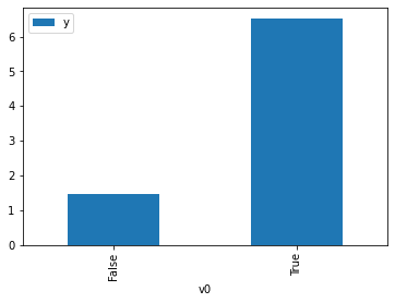
[3]:
# data['df'] is just a regular pandas.DataFrame
df.causal.do(x=treatment,
                     variable_types={treatment: 'b', outcome: 'c', common_cause: 'c'},
                     outcome=outcome,
                     common_causes=[common_cause],
                     proceed_when_unidentifiable=True).groupby(treatment).mean().plot(y=outcome, kind='bar')
[3]:
<AxesSubplot:xlabel='v0'>
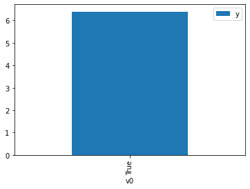
[4]:
df.causal.do(x={treatment: 1},
              variable_types={treatment:'b', outcome: 'c', common_cause: 'c'},
              outcome=outcome,
              method='weighting',
              common_causes=[common_cause],
              proceed_when_unidentifiable=True).groupby(treatment).mean().plot(y=outcome, kind='bar')
[4]:
<AxesSubplot:xlabel='v0'>
[5]:
cdf_1 = df.causal.do(x={treatment: 1},
              variable_types={treatment: 'b', outcome: 'c', common_cause: 'c'},
              outcome=outcome,
              dot_graph=data['dot_graph'],
              proceed_when_unidentifiable=True)

cdf_0 = df.causal.do(x={treatment: 0},
              variable_types={treatment: 'b', outcome: 'c', common_cause: 'c'},
              outcome=outcome,
              dot_graph=data['dot_graph'],
              proceed_when_unidentifiable=True)
[6]:
cdf_0
[6]:
| W0 | v0 | y | propensity_score | weight | |
|---|---|---|---|---|---|
| 0 | 1.117996 | False | 2.497059 | 0.333225 | 3.000976 |
| 1 | 0.238462 | False | 0.509070 | 0.455258 | 2.196556 |
| 2 | 0.213945 | False | 2.279505 | 0.458815 | 2.179528 |
| 3 | 0.425245 | False | -0.297296 | 0.428336 | 2.334615 |
| 4 | 2.301323 | False | 3.431520 | 0.200139 | 4.996525 |
| ... | ... | ... | ... | ... | ... |
| 995 | 0.621286 | False | 1.458936 | 0.400531 | 2.496683 |
| 996 | 1.642750 | False | 3.409962 | 0.268860 | 3.719407 |
| 997 | 0.409933 | False | -0.635569 | 0.430529 | 2.322722 |
| 998 | -0.063154 | False | 0.953209 | 0.499221 | 2.003123 |
| 999 | 1.532964 | False | 2.817101 | 0.281662 | 3.550353 |
1000 rows × 5 columns
[7]:
cdf_1
[7]:
| W0 | v0 | y | propensity_score | weight | |
|---|---|---|---|---|---|
| 0 | 1.055191 | True | 5.738184 | 0.658568 | 1.518446 |
| 1 | 1.676538 | True | 7.187013 | 0.735005 | 1.360535 |
| 2 | 0.111945 | True | 4.353155 | 0.526346 | 1.899889 |
| 3 | -0.840229 | True | 3.503758 | 0.389082 | 2.570151 |
| 4 | 0.556640 | True | 5.125285 | 0.590361 | 1.693878 |
| ... | ... | ... | ... | ... | ... |
| 995 | 0.018338 | True | 6.145009 | 0.512687 | 1.950507 |
| 996 | 0.094625 | True | 5.329991 | 0.523821 | 1.909048 |
| 997 | 0.711712 | True | 4.394407 | 0.612092 | 1.633741 |
| 998 | 1.928415 | True | 8.157832 | 0.762678 | 1.311169 |
| 999 | -0.280647 | True | 5.377214 | 0.469032 | 2.132052 |
1000 rows × 5 columns
Comparing the estimate to Linear Regression
First, estimating the effect using the causal data frame, and the 95% confidence interval.
[8]:
(cdf_1['y'] - cdf_0['y']).mean()
[8]:
$\displaystyle 5.092590494260132$
[9]:
1.96*(cdf_1['y'] - cdf_0['y']).std() / np.sqrt(len(df))
[9]:
$\displaystyle 0.17478007931409847$
Comparing to the estimate from OLS.
[10]:
model = OLS(np.asarray(df[outcome]), np.asarray(df[[common_cause, treatment]], dtype=np.float64))
result = model.fit()
result.summary()
[10]:
| Dep. Variable: | y | R-squared (uncentered): | 0.970 |
|---|---|---|---|
| Model: | OLS | Adj. R-squared (uncentered): | 0.970 |
| Method: | Least Squares | F-statistic: | 1.620e+04 |
| Date: | Tue, 02 Mar 2021 | Prob (F-statistic): | 0.00 |
| Time: | 20:29:26 | Log-Likelihood: | -1414.1 |
| No. Observations: | 1000 | AIC: | 2832. |
| Df Residuals: | 998 | BIC: | 2842. |
| Df Model: | 2 | ||
| Covariance Type: | nonrobust |
| coef | std err | t | P>|t| | [0.025 | 0.975] | |
|---|---|---|---|---|---|---|
| x1 | 1.7444 | 0.031 | 55.843 | 0.000 | 1.683 | 1.806 |
| x2 | 5.0338 | 0.052 | 97.742 | 0.000 | 4.933 | 5.135 |
| Omnibus: | 4.501 | Durbin-Watson: | 1.900 |
|---|---|---|---|
| Prob(Omnibus): | 0.105 | Jarque-Bera (JB): | 4.538 |
| Skew: | 0.147 | Prob(JB): | 0.103 |
| Kurtosis: | 2.851 | Cond. No. | 2.50 |
Notes:
[1] R² is computed without centering (uncentered) since the model does not contain a constant.
[2] Standard Errors assume that the covariance matrix of the errors is correctly specified.