Conditional Average Treatment Effects (CATE) with DoWhy and EconML
This is an experimental feature where we use EconML methods from DoWhy. Using EconML allows CATE estimation using different methods.
All four steps of causal inference in DoWhy remain the same: model, identify, estimate, and refute. The key difference is that we now call econml methods in the estimation step. There is also a simpler example using linear regression to understand the intuition behind CATE estimators.
All datasets are generated using linear structural equations.
[1]:
import numpy as np
import pandas as pd
import logging

import dowhy
from dowhy import CausalModel
import dowhy.datasets

import econml
import warnings
warnings.filterwarnings('ignore')

BETA = 10
[2]:
data = dowhy.datasets.linear_dataset(BETA, num_common_causes=4, num_samples=10000,
                                    num_instruments=2, num_effect_modifiers=2,
                                     num_treatments=1,
                                    treatment_is_binary=False,
                                    num_discrete_common_causes=2,
                                    num_discrete_effect_modifiers=0,
                                    one_hot_encode=False)
df=data['df']
print(df.head())
print("True causal estimate is", data["ate"])
         X0        X1   Z0        Z1        W0        W1 W2 W3         v0  \
0  1.898922 -1.493600  1.0  0.093164  0.097720  0.440277  3  2  22.528813
1  0.885180 -2.027130  0.0  0.790633  0.203576 -0.210274  2  2  16.619325
2  0.379053 -0.216526  0.0  0.049098 -0.453768 -0.439534  0  3  -1.908925
3  1.384133  1.860552  0.0  0.224985  1.216297  0.075126  1  0   7.027797
4  0.803883 -1.275331  1.0  0.511890  0.302380  1.060172  2  0  24.172841

            y
0  357.902396
1  199.083575
2  -21.889854
3  117.426939
4  296.879249
True causal estimate is 11.13817451301838
[3]:
model = CausalModel(data=data["df"],
                    treatment=data["treatment_name"], outcome=data["outcome_name"],
                    graph=data["gml_graph"])
[4]:
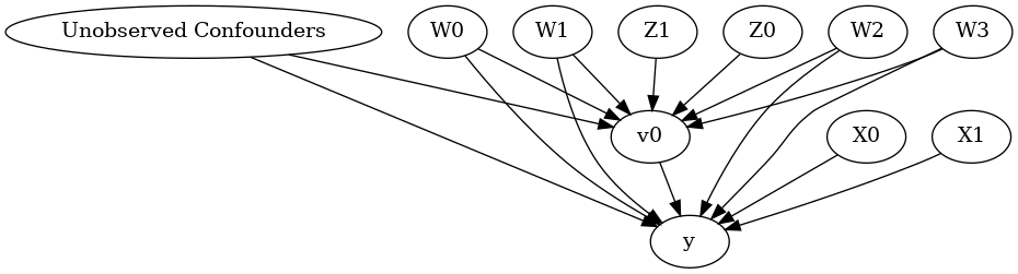
model.view_model()
from IPython.display import Image, display
display(Image(filename="causal_model.png"))
[5]:
identified_estimand= model.identify_effect(proceed_when_unidentifiable=True)
print(identified_estimand)
Estimand type: nonparametric-ate

### Estimand : 1
Estimand name: backdoor
Estimand expression:
  d
─────(Expectation(y|W3,W2,W1,X1,X0,W0))
d[v₀]
Estimand assumption 1, Unconfoundedness: If U→{v0} and U→y then P(y|v0,W3,W2,W1,X1,X0,W0,U) = P(y|v0,W3,W2,W1,X1,X0,W0)

### Estimand : 2
Estimand name: iv
Estimand expression:
Expectation(Derivative(y, [Z1, Z0])*Derivative([v0], [Z1, Z0])**(-1))
Estimand assumption 1, As-if-random: If U→→y then ¬(U →→{Z1,Z0})
Estimand assumption 2, Exclusion: If we remove {Z1,Z0}→{v0}, then ¬({Z1,Z0}→y)

### Estimand : 3
Estimand name: frontdoor
No such variable found!
Linear Model
First, let us build some intuition using a linear model for estimating CATE. The effect modifiers (that lead to a heterogeneous treatment effect) can be modeled as interaction terms with the treatment. Thus, their value modulates the effect of treatment.
Below the estimated effect of changing treatment from 0 to 1.
[6]:
linear_estimate = model.estimate_effect(identified_estimand,
                                        method_name="backdoor.linear_regression",
                                       control_value=0,
                                       treatment_value=1)
print(linear_estimate)
*** Causal Estimate ***

## Identified estimand
Estimand type: nonparametric-ate

### Estimand : 1
Estimand name: backdoor
Estimand expression:
  d
─────(Expectation(y|W3,W2,W1,X1,X0,W0))
d[v₀]
Estimand assumption 1, Unconfoundedness: If U→{v0} and U→y then P(y|v0,W3,W2,W1,X1,X0,W0,U) = P(y|v0,W3,W2,W1,X1,X0,W0)

## Realized estimand
b: y~v0+W3+W2+W1+X1+X0+W0+v0*X1+v0*X0
Target units: ate

## Estimate
Mean value: 11.138323583866043
### Conditional Estimates
__categorical__X1  __categorical__X0
(-3.742, -1.16]    (-3.816, -0.439]      5.350980
                   (-0.439, 0.172]       8.452173
                   (0.172, 0.677]       10.231967
                   (0.677, 1.246]       11.996779
                   (1.246, 4.411]       14.906734
(-1.16, -0.589]    (-3.816, -0.439]      5.981074
                   (-0.439, 0.172]       8.985925
                   (0.172, 0.677]       10.909247
                   (0.677, 1.246]       12.577942
                   (1.246, 4.411]       15.509218
(-0.589, -0.1]     (-3.816, -0.439]      6.582177
                   (-0.439, 0.172]       9.335388
                   (0.172, 0.677]       11.190280
                   (0.677, 1.246]       12.909711
                   (1.246, 4.411]       15.754069
(-0.1, 0.472]      (-3.816, -0.439]      6.810293
                   (-0.439, 0.172]       9.691918
                   (0.172, 0.677]       11.559779
                   (0.677, 1.246]       13.262256
                   (1.246, 4.411]       16.144426
(0.472, 3.296]     (-3.816, -0.439]      7.313792
                   (-0.439, 0.172]      10.285809
                   (0.172, 0.677]       12.091017
                   (0.677, 1.246]       13.846789
                   (1.246, 4.411]       16.792039
dtype: float64
EconML methods
We now move to the more advanced methods from the EconML package for estimating CATE.
First, let us look at the double machine learning estimator. Method_name corresponds to the fully qualified name of the class that we want to use. For double ML, it is “econml.dml.DML”.
Target units defines the units over which the causal estimate is to be computed. This can be a lambda function filter on the original dataframe, a new Pandas dataframe, or a string corresponding to the three main kinds of target units (“ate”, “att” and “atc”). Below we show an example of a lambda function.
Method_params are passed directly to EconML. For details on allowed parameters, refer to the EconML documentation.
[7]:
from sklearn.preprocessing import PolynomialFeatures
from sklearn.linear_model import LassoCV
from sklearn.ensemble import GradientBoostingRegressor
dml_estimate = model.estimate_effect(identified_estimand, method_name="backdoor.econml.dml.DML",
                                     control_value = 0,
                                     treatment_value = 1,
                                 target_units = lambda df: df["X0"]>1,  # condition used for CATE
                                 confidence_intervals=False,
                                method_params={"init_params":{'model_y':GradientBoostingRegressor(),
                                                              'model_t': GradientBoostingRegressor(),
                                                              "model_final":LassoCV(fit_intercept=False),
                                                              'featurizer':PolynomialFeatures(degree=1, include_bias=False)},
                                               "fit_params":{}})
print(dml_estimate)
*** Causal Estimate ***

## Identified estimand
Estimand type: nonparametric-ate

### Estimand : 1
Estimand name: backdoor
Estimand expression:
  d
─────(Expectation(y|W3,W2,W1,X1,X0,W0))
d[v₀]
Estimand assumption 1, Unconfoundedness: If U→{v0} and U→y then P(y|v0,W3,W2,W1,X1,X0,W0,U) = P(y|v0,W3,W2,W1,X1,X0,W0)

## Realized estimand
b: y~v0+W3+W2+W1+X1+X0+W0 | X1,X0
Target units: Data subset defined by a function

## Estimate
Mean value: 15.15260356848542
Effect estimates: [15.33955778 15.84879232 14.66910411 ... 18.4715256  14.39605376
 17.57646996]
[8]:
print("True causal estimate is", data["ate"])
True causal estimate is 11.13817451301838
[9]:
dml_estimate = model.estimate_effect(identified_estimand, method_name="backdoor.econml.dml.DML",
                                     control_value = 0,
                                     treatment_value = 1,
                                 target_units = 1,  # condition used for CATE
                                 confidence_intervals=False,
                                method_params={"init_params":{'model_y':GradientBoostingRegressor(),
                                                              'model_t': GradientBoostingRegressor(),
                                                              "model_final":LassoCV(fit_intercept=False),
                                                              'featurizer':PolynomialFeatures(degree=1, include_bias=True)},
                                               "fit_params":{}})
print(dml_estimate)
*** Causal Estimate ***

## Identified estimand
Estimand type: nonparametric-ate

### Estimand : 1
Estimand name: backdoor
Estimand expression:
  d
─────(Expectation(y|W3,W2,W1,X1,X0,W0))
d[v₀]
Estimand assumption 1, Unconfoundedness: If U→{v0} and U→y then P(y|v0,W3,W2,W1,X1,X0,W0,U) = P(y|v0,W3,W2,W1,X1,X0,W0)

## Realized estimand
b: y~v0+W3+W2+W1+X1+X0+W0 | X1,X0
Target units:

## Estimate
Mean value: 11.037725784237395
Effect estimates: [15.27390981 11.5084465  11.0123769  ...  7.07033426 11.24713532
 10.45835842]
CATE Object and Confidence Intervals
EconML provides its own methods to compute confidence intervals. Using BootstrapInference in the example below.
[10]:
from sklearn.preprocessing import PolynomialFeatures
from sklearn.linear_model import LassoCV
from sklearn.ensemble import GradientBoostingRegressor
from econml.inference import BootstrapInference
dml_estimate = model.estimate_effect(identified_estimand,
                                     method_name="backdoor.econml.dml.DML",
                                     target_units = "ate",
                                     confidence_intervals=True,
                                     method_params={"init_params":{'model_y':GradientBoostingRegressor(),
                                                              'model_t': GradientBoostingRegressor(),
                                                              "model_final": LassoCV(fit_intercept=False),
                                                              'featurizer':PolynomialFeatures(degree=1, include_bias=True)},
                                               "fit_params":{
                                                               'inference': BootstrapInference(n_bootstrap_samples=100, n_jobs=-1),
                                                            }
                                              })
print(dml_estimate)
*** Causal Estimate ***

## Identified estimand
Estimand type: nonparametric-ate

### Estimand : 1
Estimand name: backdoor
Estimand expression:
  d
─────(Expectation(y|W3,W2,W1,X1,X0,W0))
d[v₀]
Estimand assumption 1, Unconfoundedness: If U→{v0} and U→y then P(y|v0,W3,W2,W1,X1,X0,W0,U) = P(y|v0,W3,W2,W1,X1,X0,W0)

## Realized estimand
b: y~v0+W3+W2+W1+X1+X0+W0 | X1,X0
Target units: ate

## Estimate
Mean value: 11.03107854161636
Effect estimates: [15.23154757 11.4914362  11.00644985 ...  7.09605105 11.23996513
 10.45151404]
95.0% confidence interval: (array([15.20814535, 11.43427515, 10.97728669, ...,  6.92179496,
       11.21199051, 10.40377708]), array([15.53654796, 11.69017454, 11.10728956, ...,  7.17041884,
       11.35021865, 10.56899233]))
Can provide a new inputs as target units and estimate CATE on them.
[11]:
test_cols= data['effect_modifier_names'] # only need effect modifiers' values
test_arr = [np.random.uniform(0,1, 10) for _ in range(len(test_cols))] # all variables are sampled uniformly, sample of 10
test_df = pd.DataFrame(np.array(test_arr).transpose(), columns=test_cols)
dml_estimate = model.estimate_effect(identified_estimand,
                                     method_name="backdoor.econml.dml.DML",
                                     target_units = test_df,
                                     confidence_intervals=False,
                                     method_params={"init_params":{'model_y':GradientBoostingRegressor(),
                                                              'model_t': GradientBoostingRegressor(),
                                                              "model_final":LassoCV(),
                                                              'featurizer':PolynomialFeatures(degree=1, include_bias=True)},
                                               "fit_params":{}
                                              })
print(dml_estimate.cate_estimates)
[11.09338659 12.13565105 11.3207331  12.64976079 13.0817584  12.11993925
 11.57045914 11.44465176 13.48497597 11.05031631]
Can also retrieve the raw EconML estimator object for any further operations
[12]:
print(dml_estimate._estimator_object)
<econml.dml.dml.DML object at 0x7f516ff479d0>
Works with any EconML method
In addition to double machine learning, below we example analyses using orthogonal forests, DRLearner (bug to fix), and neural network-based instrumental variables.
Binary treatment, Binary outcome
[13]:
data_binary = dowhy.datasets.linear_dataset(BETA, num_common_causes=4, num_samples=10000,
                                    num_instruments=2, num_effect_modifiers=2,
                                    treatment_is_binary=True, outcome_is_binary=True)
# convert boolean values to {0,1} numeric
data_binary['df'].v0 = data_binary['df'].v0.astype(int)
data_binary['df'].y = data_binary['df'].y.astype(int)
print(data_binary['df'])

model_binary = CausalModel(data=data_binary["df"],
                    treatment=data_binary["treatment_name"], outcome=data_binary["outcome_name"],
                    graph=data_binary["gml_graph"])
identified_estimand_binary = model_binary.identify_effect(proceed_when_unidentifiable=True)
            X0        X1   Z0        Z1        W0        W1        W2  \
0     0.607055 -1.614792  1.0  0.455616  1.221222 -0.648731  1.326302
1     2.993224 -0.200924  0.0  0.311552 -0.804113  0.837046 -0.219313
2     1.991809  1.339323  0.0  0.177437  0.541844 -1.252206 -0.018509
3     1.375978  0.476735  1.0  0.549200 -1.052208 -1.242290  0.363920
4     0.802443 -0.904535  0.0  0.348527  1.370334 -0.536766 -0.011914
...        ...       ...  ...       ...       ...       ...       ...
9995 -0.376158 -0.719342  0.0  0.213180 -0.463657 -1.072515 -1.974591
9996  0.116404  2.395842  0.0  0.153815  1.254356 -1.060713  1.624262
9997  0.514493 -0.307350  1.0  0.048421 -0.141551  0.897432 -0.602098
9998  0.715935 -1.660456  0.0  0.895173 -0.653106  2.064832 -0.931449
9999  1.145919 -1.137355  1.0  0.068377  1.188003 -0.917376 -0.878206

            W3  v0  y
0    -0.496089   1  1
1    -0.455882   0  1
2     0.276731   1  1
3     0.027972   1  1
4    -0.133733   1  1
...        ...  .. ..
9995 -1.383749   0  0
9996 -0.553284   1  1
9997 -0.602913   1  1
9998  0.302548   1  1
9999 -0.008667   1  1

[10000 rows x 10 columns]
Using DRLearner estimator
[14]:
from sklearn.linear_model import LogisticRegressionCV
#todo needs binary y
drlearner_estimate = model_binary.estimate_effect(identified_estimand_binary,
                                method_name="backdoor.econml.drlearner.LinearDRLearner",
                                confidence_intervals=False,
                                method_params={"init_params":{
                                                    'model_propensity': LogisticRegressionCV(cv=3, solver='lbfgs', multi_class='auto')
                                                    },
                                               "fit_params":{}
                                              })
print(drlearner_estimate)
print("True causal estimate is", data_binary["ate"])
*** Causal Estimate ***

## Identified estimand
Estimand type: nonparametric-ate

### Estimand : 1
Estimand name: backdoor
Estimand expression:
  d
─────(Expectation(y|W3,W2,W1,X1,X0,W0))
d[v₀]
Estimand assumption 1, Unconfoundedness: If U→{v0} and U→y then P(y|v0,W3,W2,W1,X1,X0,W0,U) = P(y|v0,W3,W2,W1,X1,X0,W0)

## Realized estimand
b: y~v0+W3+W2+W1+X1+X0+W0 | X1,X0
Target units: ate

## Estimate
Mean value: 0.48099941411381597
Effect estimates: [0.34133643 0.58394521 0.69402234 ... 0.46721726 0.34146445 0.41183014]

True causal estimate is 0.3833
Instrumental Variable Method
[15]:
import keras
from econml.deepiv import DeepIVEstimator
dims_zx = len(model._instruments)+len(model._effect_modifiers)
dims_tx = len(model._treatment)+len(model._effect_modifiers)
treatment_model = keras.Sequential([keras.layers.Dense(128, activation='relu', input_shape=(dims_zx,)), # sum of dims of Z and X
                                    keras.layers.Dropout(0.17),
                                    keras.layers.Dense(64, activation='relu'),
                                    keras.layers.Dropout(0.17),
                                    keras.layers.Dense(32, activation='relu'),
                                    keras.layers.Dropout(0.17)])
response_model = keras.Sequential([keras.layers.Dense(128, activation='relu', input_shape=(dims_tx,)), # sum of dims of T and X
                                    keras.layers.Dropout(0.17),
                                    keras.layers.Dense(64, activation='relu'),
                                    keras.layers.Dropout(0.17),
                                    keras.layers.Dense(32, activation='relu'),
                                    keras.layers.Dropout(0.17),
                                    keras.layers.Dense(1)])

deepiv_estimate = model.estimate_effect(identified_estimand,
                                        method_name="iv.econml.deepiv.DeepIV",
                                        target_units = lambda df: df["X0"]>-1,
                                        confidence_intervals=False,
                                method_params={"init_params":{'n_components': 10, # Number of gaussians in the mixture density networks
                                                              'm': lambda z, x: treatment_model(keras.layers.concatenate([z, x])), # Treatment model,
                                                              "h": lambda t, x: response_model(keras.layers.concatenate([t, x])), # Response model
                                                              'n_samples': 1, # Number of samples used to estimate the response
                                                              'first_stage_options': {'epochs':25},
                                                              'second_stage_options': {'epochs':25}
                                                             },
                                               "fit_params":{}})
print(deepiv_estimate)
Using TensorFlow backend.
Epoch 1/25
10000/10000 [==============================] - 2s 158us/step - loss: 6.0581
Epoch 2/25
10000/10000 [==============================] - 1s 90us/step - loss: 2.5423
Epoch 3/25
10000/10000 [==============================] - 1s 88us/step - loss: 2.3626
Epoch 4/25
10000/10000 [==============================] - 1s 87us/step - loss: 2.3099
Epoch 5/25
10000/10000 [==============================] - 1s 87us/step - loss: 2.2638
Epoch 6/25
10000/10000 [==============================] - 1s 99us/step - loss: 2.2351
Epoch 7/25
10000/10000 [==============================] - 1s 94us/step - loss: 2.2353
Epoch 8/25
10000/10000 [==============================] - 1s 83us/step - loss: 2.2118
Epoch 9/25
10000/10000 [==============================] - 1s 84us/step - loss: 2.2095
Epoch 10/25
10000/10000 [==============================] - 1s 83us/step - loss: 2.1964
Epoch 11/25
10000/10000 [==============================] - 1s 83us/step - loss: 2.1899
Epoch 12/25
10000/10000 [==============================] - 1s 99us/step - loss: 2.1810
Epoch 13/25
10000/10000 [==============================] - 1s 110us/step - loss: 2.1768
Epoch 14/25
10000/10000 [==============================] - 1s 107us/step - loss: 2.1662
Epoch 15/25
10000/10000 [==============================] - 1s 97us/step - loss: 2.1600
Epoch 16/25
10000/10000 [==============================] - 1s 81us/step - loss: 2.1619
Epoch 17/25
10000/10000 [==============================] - 1s 89us/step - loss: 2.1534
Epoch 18/25
10000/10000 [==============================] - 1s 105us/step - loss: 2.1529
Epoch 19/25
10000/10000 [==============================] - 1s 96us/step - loss: 2.1530
Epoch 20/25
10000/10000 [==============================] - 1s 104us/step - loss: 2.1509
Epoch 21/25
10000/10000 [==============================] - 1s 91us/step - loss: 2.1388
Epoch 22/25
10000/10000 [==============================] - 1s 88us/step - loss: 2.1440
Epoch 23/25
10000/10000 [==============================] - 1s 87us/step - loss: 2.1422
Epoch 24/25
10000/10000 [==============================] - 1s 94us/step - loss: 2.1302
Epoch 25/25
10000/10000 [==============================] - 1s 92us/step - loss: 2.1334
Epoch 1/25
10000/10000 [==============================] - 2s 197us/step - loss: 9634.7153
Epoch 2/25
10000/10000 [==============================] - 1s 124us/step - loss: 6117.5493
Epoch 3/25
10000/10000 [==============================] - 1s 132us/step - loss: 6080.0172
Epoch 4/25
10000/10000 [==============================] - 1s 144us/step - loss: 6000.0626
Epoch 5/25
10000/10000 [==============================] - 1s 140us/step - loss: 5903.0761
Epoch 6/25
10000/10000 [==============================] - 1s 114us/step - loss: 5971.7064
Epoch 7/25
10000/10000 [==============================] - 1s 109us/step - loss: 5927.9321
Epoch 8/25
10000/10000 [==============================] - 1s 107us/step - loss: 6042.7108
Epoch 9/25
10000/10000 [==============================] - 1s 107us/step - loss: 5935.9766
Epoch 10/25
10000/10000 [==============================] - 1s 108us/step - loss: 5899.0229
Epoch 11/25
10000/10000 [==============================] - 1s 108us/step - loss: 5814.6864
Epoch 12/25
10000/10000 [==============================] - 1s 110us/step - loss: 5938.3598
Epoch 13/25
10000/10000 [==============================] - 1s 110us/step - loss: 5783.8304
Epoch 14/25
10000/10000 [==============================] - 1s 110us/step - loss: 5861.9487
Epoch 15/25
10000/10000 [==============================] - 1s 122us/step - loss: 5884.3656
Epoch 16/25
10000/10000 [==============================] - 1s 145us/step - loss: 5875.7650
Epoch 17/25
10000/10000 [==============================] - 1s 131us/step - loss: 5842.4607
Epoch 18/25
10000/10000 [==============================] - 1s 117us/step - loss: 5833.5643
Epoch 19/25
10000/10000 [==============================] - 1s 123us/step - loss: 5883.4645
Epoch 20/25
10000/10000 [==============================] - 1s 110us/step - loss: 5888.1516
Epoch 21/25
10000/10000 [==============================] - 1s 111us/step - loss: 5883.6870
Epoch 22/25
10000/10000 [==============================] - 1s 111us/step - loss: 5917.5608
Epoch 23/25
10000/10000 [==============================] - 1s 114us/step - loss: 5954.1094
Epoch 24/25
10000/10000 [==============================] - 1s 110us/step - loss: 5871.8566
Epoch 25/25
10000/10000 [==============================] - 1s 117us/step - loss: 5842.7111
*** Causal Estimate ***

## Identified estimand
Estimand type: nonparametric-ate

### Estimand : 1
Estimand name: iv
Estimand expression:
Expectation(Derivative(y, [Z1, Z0])*Derivative([v0], [Z1, Z0])**(-1))
Estimand assumption 1, As-if-random: If U→→y then ¬(U →→{Z1,Z0})
Estimand assumption 2, Exclusion: If we remove {Z1,Z0}→{v0}, then ¬({Z1,Z0}→y)

## Realized estimand
b: y~v0+W3+W2+W1+X1+X0+W0 | X1,X0
Target units: Data subset defined by a function

## Estimate
Mean value: 3.3913748264312744
Effect estimates: [4.111145  2.1927567 4.0210876 ... 0.9122124 4.053177  2.2825317]
Metalearners
[16]:
data_experiment = dowhy.datasets.linear_dataset(BETA, num_common_causes=5, num_samples=10000,
                                    num_instruments=2, num_effect_modifiers=5,
                                    treatment_is_binary=True, outcome_is_binary=False)
# convert boolean values to {0,1} numeric
data_experiment['df'].v0 = data_experiment['df'].v0.astype(int)
print(data_experiment['df'])
model_experiment = CausalModel(data=data_experiment["df"],
                    treatment=data_experiment["treatment_name"], outcome=data_experiment["outcome_name"],
                    graph=data_experiment["gml_graph"])
identified_estimand_experiment = model_experiment.identify_effect(proceed_when_unidentifiable=True)
            X0        X1        X2        X3        X4   Z0        Z1  \
0    -1.511404 -0.796794  0.381156  0.546913  0.988627  1.0  0.945576
1     1.084781 -1.922791 -0.461289 -0.208160 -1.362516  0.0  0.631043
2    -0.993879  0.264821  2.495885  0.768880 -0.200069  1.0  0.564980
3    -2.752826 -1.278350  2.013659  0.225430 -0.296333  1.0  0.729429
4    -0.176540 -0.143080 -1.994730  1.445114 -1.310322  0.0  0.660578
...        ...       ...       ...       ...       ...  ...       ...
9995 -0.615514 -0.054405 -1.403155  0.047062  0.668092  0.0  0.049970
9996 -0.079075 -1.970365  0.590612  0.129645  1.702936  0.0  0.006828
9997 -0.612788 -1.583195 -0.955393  0.139663  0.633461  0.0  0.622620
9998 -2.649140 -1.605903 -1.236836 -1.253810 -1.396432  0.0  0.394677
9999 -1.006696  0.406869 -0.687812  0.247259  0.680919  0.0  0.069656

            W0        W1        W2        W3        W4  v0          y
0     0.083088 -0.950762  0.474662  1.346305 -1.790676   1   1.968666
1    -0.082310 -0.659660  1.051546  1.581745  0.195329   1  10.434861
2     1.221314 -0.894577  0.308504 -0.166613 -1.599631   1  13.105967
3     1.151428 -1.390558  2.628862  0.928396 -0.477143   1   5.665644
4     0.299112 -0.227596  1.117443  0.333261  0.822112   1   9.385864
...        ...       ...       ...       ...       ...  ..        ...
9995  0.688683 -1.733233  1.168689 -0.755424 -0.560150   0  -1.992805
9996 -0.396265  1.375946  0.622630  1.124654  0.143208   1  14.094986
9997  0.726669 -0.896359  2.831088  1.560724 -1.672692   1   8.784501
9998 -0.738313 -1.374355  1.775307  0.559349 -1.305286   1 -10.959509
9999  1.175807 -0.233245  2.094218 -0.437447 -0.219961   1  13.028082

[10000 rows x 14 columns]
[17]:
from sklearn.ensemble import RandomForestRegressor
metalearner_estimate = model_experiment.estimate_effect(identified_estimand_experiment,
                                method_name="backdoor.econml.metalearners.TLearner",
                                confidence_intervals=False,
                                method_params={"init_params":{
                                                    'models': RandomForestRegressor()
                                                    },
                                               "fit_params":{}
                                              })
print(metalearner_estimate)
print("True causal estimate is", data_experiment["ate"])
*** Causal Estimate ***

## Identified estimand
Estimand type: nonparametric-ate

### Estimand : 1
Estimand name: backdoor
Estimand expression:
  d
─────(Expectation(y|W3,W2,X4,W1,X3,X1,X2,W4,X0,W0))
d[v₀]
Estimand assumption 1, Unconfoundedness: If U→{v0} and U→y then P(y|v0,W3,W2,X4,W1,X3,X1,X2,W4,X0,W0,U) = P(y|v0,W3,W2,X4,W1,X3,X1,X2,W4,X0,W0)

## Realized estimand
b: y~v0+X3+X2+X1+X4+X0+W3+W2+W1+W4+W0
Target units: ate

## Estimate
Mean value: 6.287323303624039
Effect estimates: [ 4.61465613 12.53217671  8.69905637 ...  6.04112821 -3.265252
  6.54000794]

True causal estimate is 5.535602451644429
Refuting the estimate
Adding a random common cause variable
[18]:
res_random=model.refute_estimate(identified_estimand, dml_estimate, method_name="random_common_cause")
print(res_random)
Refute: Add a Random Common Cause
Estimated effect:11.995163235677346
New effect:12.028609904102334
Adding an unobserved common cause variable
[19]:
res_unobserved=model.refute_estimate(identified_estimand, dml_estimate, method_name="add_unobserved_common_cause",
                                     confounders_effect_on_treatment="linear", confounders_effect_on_outcome="linear",
                                    effect_strength_on_treatment=0.01, effect_strength_on_outcome=0.02)
print(res_unobserved)
Refute: Add an Unobserved Common Cause
Estimated effect:11.995163235677346
New effect:12.046656228321476
Replacing treatment with a random (placebo) variable
[20]:
res_placebo=model.refute_estimate(identified_estimand, dml_estimate,
        method_name="placebo_treatment_refuter", placebo_type="permute",
        num_simulations=10 # at least 100 is good, setting to 10 for speed
        )
print(res_placebo)
Refute: Use a Placebo Treatment
Estimated effect:11.995163235677346
New effect:0.014174758181060527
p value:0.40645666707426864
Removing a random subset of the data
[21]:
res_subset=model.refute_estimate(identified_estimand, dml_estimate,
        method_name="data_subset_refuter", subset_fraction=0.8,
        num_simulations=10)
print(res_subset)
Refute: Use a subset of data
Estimated effect:11.995163235677346
New effect:11.998974744372351
p value:0.46530895233272207
More refutation methods to come, especially specific to the CATE estimators.