Direct Effect: Quantifying Arrow Strength
By quantifying the strength of an arrow, we answer the question:
How strong is the causal influence from a cause to its direct effect?
While there are different definitions for measuring causal influences in the literature, DoWhy offers an implementation for measuring the direct influence of a parent node on a child, where influences through paths over other nodes are ignored. This method is based on the paper:
Dominik Janzing, David Balduzzi, Moritz Grosse-Wentrup, Bernhard Schölkopf. Quantifying causal influences The Annals of Statistics, Vol. 41, No. 5, 2324-2358, 2013.
How to use it
To see how to use the method, let us generate some data.
>>> import numpy as np, pandas as pd, networkx as nx
>>> from dowhy import gcm
>>> np.random.seed(10)  # to reproduce these results
>>> Z = np.random.normal(loc=0, scale=1, size=1000)
>>> X = 2*Z + np.random.normal(loc=0, scale=1, size=1000)
>>> Y = 3*X + 4*Z + np.random.normal(loc=0, scale=1, size=1000)
>>> data = pd.DataFrame(dict(X=X, Y=Y, Z=Z))
Next, we will model cause-effect relationships as a probabilistic causal model and fit it to the data.
>>> causal_model = gcm.ProbabilisticCausalModel(nx.DiGraph([('Z', 'Y'), ('Z', 'X'), ('X', 'Y')]))
>>> causal_model.set_causal_mechanism('Z', gcm.EmpiricalDistribution())
>>> causal_model.set_causal_mechanism('X', gcm.AdditiveNoiseModel(gcm.ml.create_linear_regressor()))
>>> causal_model.set_causal_mechanism('Y', gcm.AdditiveNoiseModel(gcm.ml.create_linear_regressor()))
>>> gcm.fit(causal_model, data)
Finally, we can estimate the strength of incoming arrows to a node of interest (e.g., \(Y\)).
>>> strength = gcm.arrow_strength(causal_model, 'Y')
>>> strength
    {('X', 'Y'): 41.321925893102716,
     ('Z', 'Y'): 14.736197949517237}
Interpreting the results: By default, the measurement unit of the scalar values for arrow strengths is variance for a continuous real-valued target, and the number of bits for a categorical target (i.e., KL divergence). Above, we observe that the direct influence from \(X\) to \(Y\) (~41.32) is stronger (by ~2.7 times) than the direct influence from \(Z\) to \(Y\) (~14.73). Roughly speaking, “removing” the arrow from \(X\) to \(Y\) increases the variance of \(Y\) by ~41.32 units, whereas removing \(Z \to Y\) increases the variance of \(Y\) by ~14.73 units.
In the next section, we explain what “removing” an edge implies. In particular, we briefly explain the science behind our method for quantifying the strength of an arrow.
Understanding the method
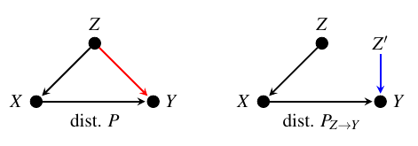
We will use the causal graph below to illustrate the key idea behind the method.

Here, we want to measure the strength of the arrow from node \(Z\) to node \(Y\), while disregarding any indirect effects via \(X\). To achieve this, first recall that we can obtain the joint distribution of variables \(P\) from their causal graph via a product of conditional distributions of each variable given its parents.
We then create a new joint distribution \(P_{Z \to Y}\) by cutting the edge from \(Z\) to \(Y\) and using an i.i.d. copy of \(Z\) (denoted as \(Z'\) in the figure) instead as input to \(Y\). The distribution of \(Z'\) can be practically simulated by randomly shuffling the observed values of \(Z\). The strength of the arrow from \(Z\) to \(Y\), represented as \(C_{Z \to Y}\), is then calculated as the distance between the post-cutting distribution:math:P_{Z to Y} and the original joint distribution \(P\):
The distance metric \(D\) utilized to calculate the arrow strength can be any suitable measure, such as the difference of variances or KL divergence. By default, the library uses a specific measure depending on the data type, but this can be fully customized to the use case.
Note that when cutting the edge, only the causal mechanism of the target variable changes between the original and post-cutting joint distribution. As a result, any change in the marginal distribution of the target is due to the change in the causal mechanism of the target. This allows us to also quantify the arrow strength in terms of the change in the property (e.g., variance) of the marginal distribution of the target when we remove an edge.
Customize the distance measure
By default, arrow_strength uses the difference of variances for measuring the arrow strength for a continuous real-valued target and employs
KL divergence for measuring the arrow strength for a categorical target. But, we can also plug in our own choice of measure, using the
difference_estimation_func parameter. For instance, to measure the arrow strength in terms of the change in the mean, we could
define:
>>> def mean_diff(Y_old, Y_new): return np.mean(Y_new) - np.mean(Y_old)
and then estimate the arrow strength:
>>> gcm.arrow_strength(causal_model, 'Y', difference_estimation_func=mean_diff)
    {('X', 'Y'): 0.11898914602350251,
     ('Z', 'Y'): 0.07811542095834415}
These small results here are expected; in our example, the mean value of \(Y\) remains \(0\) regardless of whether we remove an incoming arrow. As such, the strength of incoming arrows to \(Y\) with respect to their influence on the mean should be negligible.
In summary, arrow strength can be measured in different units (e.g., mean, variance, bits). Therefore, we advise users to pick a meaningful unit—based on data and interpretation—to apply this method in practice.