Order-based algorithms for causal discovery from observational data without latent confounders

We will simulate some observational data from a Structural Causal Model (SCM) and demonstrate how we will use the SCORE algorithm. The example can be easily adapted to CAM, DAS and NoGAM methods.

CAM, SCORE, DAS, NoGAM algorithms perform causal discovery in a two steps procedure. Given observational i.i.d. data from an Additive Noise Model without latent confounders, first the method estimates a topological ordering of the causal variables. This partial ordering can be represented as a fully connected graph, where every node has an incoming edge from all its predecessors in the ordering. Second, the resulting fully connected DAG is pruned by some variable selection procedure. Note that knowing the topological ordering is already sufficient for estimating causal effects. Nevertheless, the pruning step is justified by the fact that operating with a sparser graph is statistically more efficient.

The four methods differ as follow:

• In CAM algorithm the topological ordering is inferred by finding the permutation of the graph nodes corresponding to the fully connected graph that maximizes the log-likelihood of the data. After inference of the topological ordering, the pruning step is done by variable selection with regression. In particular, for each variable j CAM fits a generalized additive model using as covariates all the predecessor of j in the ordering, and performs hypothesis testing to select relevant parent variables.

• SCORE provides a more efficient topological ordering than CAM, while it inherits the pruning procedure. In order to infer the topological ordering, SCORE estimates the Hessian matrix of the log-likelihood. Then, it finds a leaf (i.e. a node without children) by taking the argmin of the variance over the diagonal elements of the Hessian matrix. Once a leaf is found, it is removed from the graph and the procedure is iteratively repeated, evantually assigning a position to each node.

• DAS provides a more efficient pruning step, while it inherits the ordering method from SCORE. Let H be the Hessian matrix of the log-likelihood: given a leaf node j, DAS selects an edge i -> j if the pair satisfies mean(abs(H[i, j])) = 0. Vanishing mean is verified by hypothesis testing. Finally, CAM-pruning is applied on the resulting sparse graph, in order to further reduce the number of false positives in the inferred DAG. Sparsity ensures linear computational complexity of this final pruning step. (DAS can be seen as an efficient version of SCORE, with better scaling properties in the graph size.)

• NoGAM introduces a topological ordering procedure that does not assume any distribution of the noise terms, whereas CAM, SCORE and DAS all require the noise to be Gaussian. The pruning of the graph is done via CAM procedure. In order to define the topological order, NoGAM identifies one leaf at the time: first, for each node in the graph, it estimates the residuals of the regression problem that predicts a variable j from all the remaining nodes 1, 2, .., j-1, j+1, .., |V| (with |V| the number of nodes). Then, NoGAM tries to estimate each entry j of the vector of the gradient of log-likelihood using the residual of the variable j as covariate: a leaf is found by selection of the argmin of the mean squared error of the predictions.

Authors: Francesco Montagna <francesco.montagna997@gmail.com>

License: BSD (3-clause)

import numpy as np
import networkx as nx
from scipy import stats
import pandas as pd
from pywhy_graphs.viz import draw
from dodiscover import make_context
from dodiscover.toporder.score import SCORE
from dowhy import gcm
from dowhy.gcm.util.general import set_random_seed

Simulate some data

First we will simulate data, starting from an Additive Noise Model (ANM). This will then induce a causal graph, which we can visualize.

# set a random seed to make example reproducible
seed = 12345
rng = np.random.RandomState(seed=seed)


class MyCustomModel(gcm.PredictionModel):
    def __init__(self, coefficient):
        self.coefficient = coefficient

    def fit(self, X, Y):
        # Nothing to fit here, since we know the ground truth.
        pass

    def predict(self, X):
        return self.coefficient * X

    def clone(self):
        # We don't really need this actually.
        return MyCustomModel(self.coefficient)


# set a random seed to make example reproducible
set_random_seed(1234)

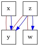
# construct a causal graph that will result in
# x -> y <- z -> w
G = nx.DiGraph([("x", "y"), ("z", "y"), ("z", "w")])

causal_model = gcm.ProbabilisticCausalModel(G)
causal_model.set_causal_mechanism("x", gcm.ScipyDistribution(stats.binom, p=0.5, n=1))
causal_model.set_causal_mechanism("z", gcm.ScipyDistribution(stats.binom, p=0.9, n=1))
causal_model.set_causal_mechanism(
    "y",
    gcm.AdditiveNoiseModel(
        prediction_model=MyCustomModel(1),
        noise_model=gcm.ScipyDistribution(stats.binom, p=0.8, n=1),
    ),
)
causal_model.set_causal_mechanism(
    "w",
    gcm.AdditiveNoiseModel(
        prediction_model=MyCustomModel(1),
        noise_model=gcm.ScipyDistribution(stats.binom, p=0.5, n=1),
    ),
)

# Fit here would not really fit parameters, since we don't do anything in the fit method.
# Here, we only need this to ensure that each FCM has the correct local hash (i.e., we
# get an inconsistency error if we would modify the graph afterwards without updating
# the FCMs). Having an empty data set is a small workaround, since all models are
# pre-defined.
gcm.fit(causal_model, pd.DataFrame(columns=["x", "y", "z", "w"]))

# sample the observational data
data = gcm.draw_samples(causal_model, num_samples=500)

print(data.head())
print(pd.Series({col: data[col].unique() for col in data}))
dot_graph = draw(G)
dot_graph.render(outfile="oracle_dag.png", view=True)

Fitting causal models:   0%|          | 0/4 [00:00<?, ?it/s]
Fitting causal mechanism of node x:   0%|          | 0/4 [00:00<?, ?it/s]
Fitting causal mechanism of node y:   0%|          | 0/4 [00:00<?, ?it/s]
Fitting causal mechanism of node z:   0%|          | 0/4 [00:00<?, ?it/s]
Fitting causal mechanism of node w:   0%|          | 0/4 [00:00<?, ?it/s]
Fitting causal mechanism of node w: 100%|##########| 4/4 [00:00<00:00, 1884.87it/s]
   x  ...  w
0  0  ...  1
1  1  ...  2
2  0  ...  1
3  1  ...  1
4  1  ...  1

[5 rows x 4 columns]
x       [0, 1]
z       [1, 0]
y    [1, 2, 0]
w    [1, 2, 0]
dtype: object

'oracle_dag.png'

Define the context

In PyWhy, we introduce the context.Context class, which should be a departure from “data-first causal discovery,” where users provide data as the primary input to a discovery algorithm. This problem with this approach is that it encourages novice users to see the algorithm as a philosopher’s stone that converts data to causal relationships. With this mindset, users tend to surrender the task of providing domain-specific assumptions that enable identifiability to the algorithm. In contrast, PyWhy’s key strength is how it guides users to specifying domain assumptions up front (in the form of a DAG) before the data is added, and then addresses identifiability given those assumptions and data. In this sense, the Context class houses both data, apriori assumptions and other relevant data that may be used in downstream structure learning algorithms.

context = make_context().variables(data=data).build()

# Alternatively, one could specify some fixed edges.

# .. code-block::Python
#   included_edges = nx.Graph([('x', 'y')])
#   context = make_context().edges(include=included_edges).build()

Run structure learning algorithm

Now we are ready to run the SCORE algorithm. The method performs inference in two phases. First it estimates the topological order of the nodes in the graphs. This is done iteratively according to the following procedure:

1. SCORE estimates the Hessian of the logarithm of \(p(V)\), with \(p(V)\) the joint distribution of the nodes in the graph.

2. Let H := Hessian(log p(V)). SCORE selects a leaf in the graph by finding the diagonal term of H with minimum variance, i.e. by computing np.argmin(np.var(np.diag(H)).

3. SCORE removes the leaf from the graph, and repeats steps from 1. to 3. iteratively up to the source nodes.

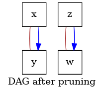
Given the inferred topological order, SCORE prunes the graph with all the edges admitted by such ordering, by doing sparse regression to choose the relevant variables. Variable selection is done by thresholding on the p-values of the coefficients associated to the potential parents of a node. For instance, consider a graph \(G\) with 3 vertices \(V = \{1, 2, 3\}\). For simplicity let the topological order be trivial, i.e. \(\{1, 2, 3\}\). The unique fully connected adjacency matrix compatible with such ordering is the upper triangular matrix np.triu(np.ones((3, 3)), k=1) with all ones above the diagonal.

score = SCORE()  # or DAS() or NoGAM() or CAM()
score.learn_graph(data, context)

# SCORE estimates a directed acyclic graph (DAG) and the topoological order
# of the nodes in the graph. SCORE is consistent in the infinite samples
# limit, meaning that it might return faulty estimates due to the finiteness
# of the data.
graph = score.graph_
order_graph = score.order_graph_

# `score_full_dag.png` visualizes the fully connected DAG representation of
# the inferred topological ordering.
# `score_dag.png` visualizes the fully connected DAG after pruning with
# sparse regression.
dot_graph = draw(graph, name="DAG after pruning")
dot_graph.render(outfile="score_dag.png", view=True)

dot_graph = draw(order_graph, name="Fully connected DAG")
dot_graph.render(outfile="score_full_dag.png", view=True)

• 
• 

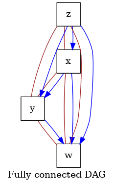
'score_full_dag.png'

Summary

We observe two DAGs output of the SCORE inference procedure. One is the fully connected graph associated to the inferred topological order [z, x, y, w] of the graph nodes. The other is the sparser graph after the pruning step, corresponding to the causal graph inferred by SCORE.