Causal discovery with interventional data - Sachs dataset

We will analyze the Sachs dataset [1] and reproduce analyses from the Supplemental Figure 8 in [2] demonstrating the usage of the dodiscover.constraint.PsiFCI algorithm for learning causal graphs from observational and/or interventional data.

The Sachs dataset is a famous dataset in causal discovery because of its real-life applicability and access to experimental data that analyzed the causal network of protein signaling pathways. We will analyze the preprocessed interventional dataset, which we download using the package pooch. The preprocessed dataset consists of categorical features, so we will use the dodiscover.ci.GSquareCITest for testing conditional independence and invariances of the conditional distributions across experimental conditions. There are a total of 6 experimental conditions represented by the INT column.

Authors: Adam Li <adam2392@gmail.com>

License: BSD (3-clause)

from pywhy_graphs.viz import draw
from dodiscover.ci import GSquareCITest
from dodiscover import PsiFCI, Context, make_context, InterventionalContextBuilder

import pandas as pd
import bnlearn

import pooch

Pull in the Sachs Dataset

The Sachs dataset is a famous dataset in causal discovery because of its real-life applicability and access to experimental data that analyzed the causal network of 11 proteins using knockouts and spikings [1]. The pathways for those proteins are already known, so it is an ideal dataset for benchmarking causal discovery algorithms.

We will download a preprocessed version of the dataset from the following url: https://www.bnlearn.com/book-crc/code/sachs.interventional.txt.gz

Ref: https://erdogant.github.io/bnlearn/pages/html/bnlearn.bnlearn.html#bnlearn.bnlearn.import_example # noqa

# use pooch to download robustly from a url
url = "https://www.bnlearn.com/book-crc/code/sachs.interventional.txt.gz"
file_path = pooch.retrieve(
    url=url,
    known_hash="md5:39ee257f7eeb94cb60e6177cf80c9544",
)

df = pd.read_csv(file_path, delimiter=" ")

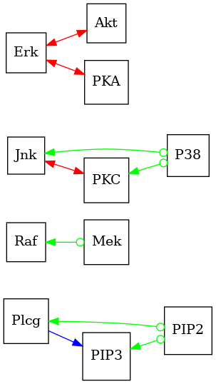
# the ground-truth dag is shown here: XXX: comment in when errors are fixed
ground_truth_dag = bnlearn.import_DAG("sachs", verbose=False)
fig = bnlearn.plot(ground_truth_dag)

# .. note::
#    The Sachs dataset has previously been preprocessed, and the steps are described
#    in bnlearn, at the web-page https://www.bnlearn.com/research/sachs05/.
print(df.head())
print(df.shape)

Downloading data from 'https://www.bnlearn.com/book-crc/code/sachs.interventional.txt.gz' to file '/home/circleci/.cache/pooch/08b7ab6b909b20c5ff42bc7d7721556c-sachs.interventional.txt.gz'.
[bnlearn] >Downloading example [sachs] dataset..
[bnlearn] >Set node properties.
[bnlearn] >Set edge properties.
[bnlearn] >Plot based on Bayesian model
   Raf  ...  INT
0    1  ...    8
1    1  ...    8
2    1  ...    8
3    1  ...    8
4    1  ...    8

[5 rows x 12 columns]
(5400, 12)

Preprocess the dataset

Since the data is one dataframe, we need to process it into a form that is acceptable by dodiscover’s constraint.PsiFCI algorithm. We will form a list of separate dataframes.

unique_ints = df["INT"].unique()

# get the list of intervention targets and list of dataframe associated with each intervention
intervention_targets = [df.columns[idx] for idx in unique_ints]
data_cols = [col for col in df.columns if col != "INT"]
data = []
for interv_idx in unique_ints:
    _data = df[df["INT"] == interv_idx][data_cols]
    data.append(_data)

print(len(data), len(intervention_targets))

6 6

Setup constraint-based learner

Since we have access to interventional data, the causal discovery algorithm we will use that leverages CI and CD tests to estimate causal constraints is the Psi-FCI algorithm [2].

# Our dataset is comprised of discrete valued data, so we will utilize the
# G^2 (Chi-square) CI test.
ci_estimator = GSquareCITest(data_type="discrete")

# Since our data is entirely discrete, we can also use the G^2 test as our
# CD test.
cd_estimator = GSquareCITest(data_type="discrete")

alpha = 0.05
learner = PsiFCI(
    ci_estimator=ci_estimator,
    cd_estimator=cd_estimator,
    alpha=alpha,
    max_combinations=10,
    max_cond_set_size=4,
    n_jobs=-1,
)

# create context with information about the interventions
ctx_builder = make_context(create_using=InterventionalContextBuilder)
ctx: Context = (
    ctx_builder.variables(data=data[0]).num_distributions(6).obs_distribution(False).build()
)

print(ctx.init_graph)
print(ctx.f_nodes)

Graph with 26 nodes and 325 edges
[('F', 0), ('F', 1), ('F', 2), ('F', 3), ('F', 4), ('F', 5), ('F', 6), ('F', 7), ('F', 8), ('F', 9), ('F', 10), ('F', 11), ('F', 12), ('F', 13), ('F', 14)]

Run the learning process

We have setup our causal context and causal discovery learner, so we will now run the algorithm using the constraint.PsiFCI.learn_graph() API, which is similar to scikit-learn’s fit design. All fitted attributes contain an underscore at the end.

learner = learner.learn_graph(data, ctx)

Analyze the results

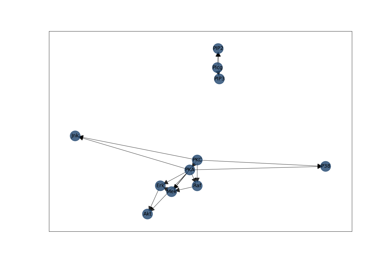
Now that we have learned the graph, we will show it here. Note differences and similarities to the ground-truth DAG that is “assumed”. Moreover, note that this reproduces Supplementary Figure 8 in [2].

est_pag = learner.graph_

print(f"There are {len(est_pag.to_undirected().edges)} edges in the resulting PAG")

There are 154 edges in the resulting PAG

Visualize the full graph including the F-node

dot_graph = draw(est_pag, direction="LR")
dot_graph.render(outfile="psi_pag_full.png", view=True, cleanup=True)

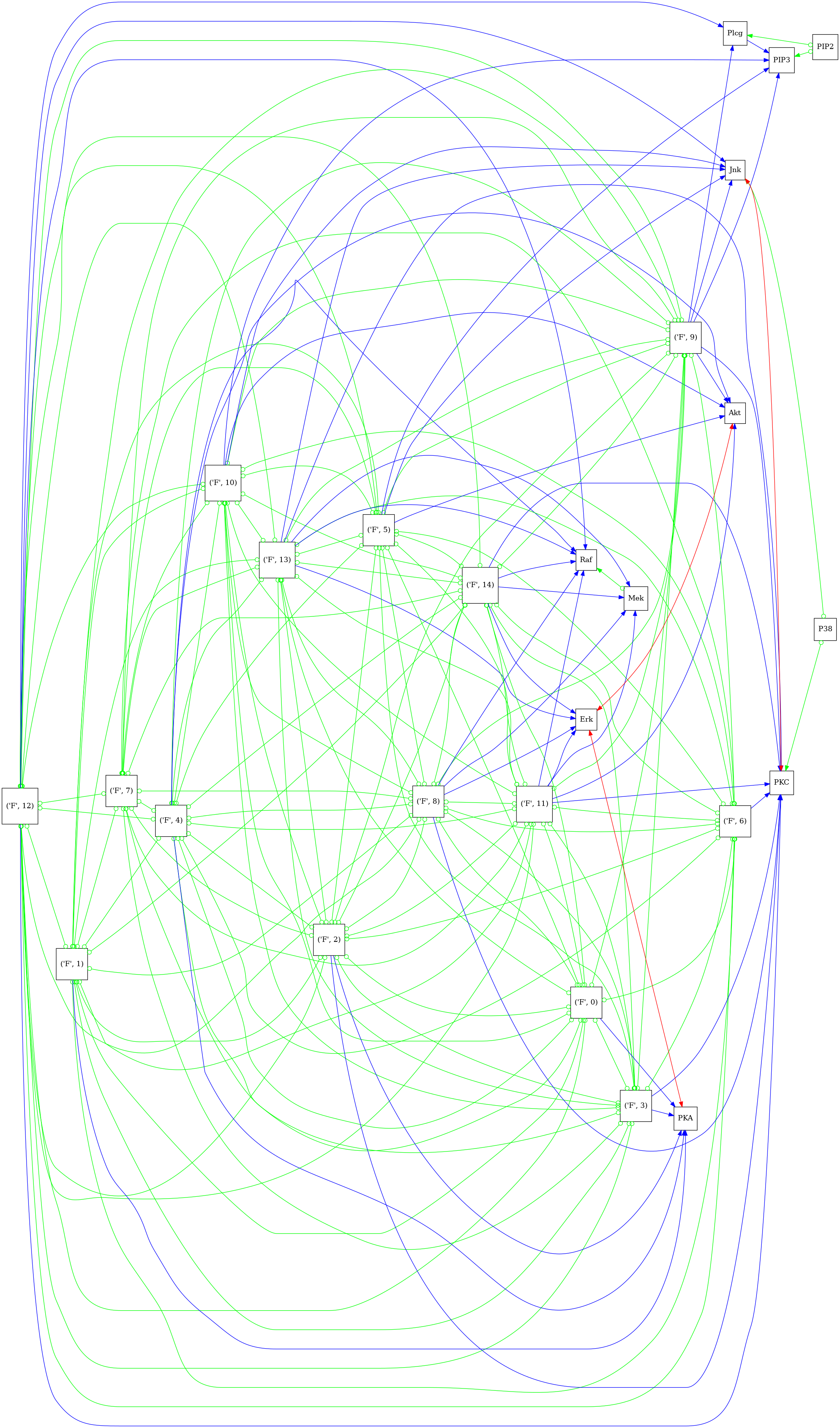
'psi_pag_full.png'

Visualize the graph without the F-nodes

est_pag_no_fnodes = est_pag.subgraph(ctx.get_non_augmented_nodes())
dot_graph = draw(est_pag_no_fnodes, direction="LR")
dot_graph.render(outfile="psi_pag.png", view=True, cleanup=True)

# Interpretation
# --------------
# Looking at the supplemental figure 8b in :footcite:`Jaber2020causal`, we see that the
# learned PAG matches quite well.

# References
# ----------
# .. footbibliography::

'psi_pag.png'