Basic causal discovery with DoDiscover using the PC algorithm

We will simulate some observational data from a Structural Causal Model (SCM) and demonstrate how we will use the PC algorithm.

The PC algorithm works on observational data when there are no unobserved latent confounders. That means for any observed set of variables, there is no common causes that are unobserved. In other words, all exogenous variables then are assumed to be independent.

In this example, we will introduce the main abstractions and concepts used in dodiscover for causal discovery:

• learner: Any causal discovery algorithm that has a similar scikit-learn API.

• context: Causal assumptions.

Authors: Adam Li <adam2392@gmail.com>

License: BSD (3-clause)

import numpy as np
import networkx as nx
from scipy import stats
from pywhy_graphs.viz import draw
from dodiscover.ci import GSquareCITest, Oracle
from dodiscover import PC, make_context
import pandas as pd
from dowhy import gcm
from dowhy.gcm.util.general import set_random_seed

Simulate some data

First we will simulate data, starting from a Structural Causal Model (SCM). This will then induce a causal graph, which we can visualize. Due to the Markov assumption, then we can use d-separation to examine which variables are conditionally independent.

# set a random seed to make example reproducible
seed = 12345
rng = np.random.RandomState(seed=seed)


class MyCustomModel(gcm.PredictionModel):
    def __init__(self, coefficient):
        self.coefficient = coefficient

    def fit(self, X, Y):
        # Nothing to fit here, since we know the ground truth.
        pass

    def predict(self, X):
        return self.coefficient * X

    def clone(self):
        # We don't really need this actually.
        return MyCustomModel(self.coefficient)


# set a random seed to make example reproducible
set_random_seed(1234)

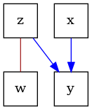
# construct a causal graph that will result in
# x -> y <- z -> w
G = nx.DiGraph([("x", "y"), ("z", "y"), ("z", "w")])

causal_model = gcm.ProbabilisticCausalModel(G)
causal_model.set_causal_mechanism("x", gcm.ScipyDistribution(stats.binom, p=0.5, n=1))
causal_model.set_causal_mechanism("z", gcm.ScipyDistribution(stats.binom, p=0.9, n=1))
causal_model.set_causal_mechanism(
    "y",
    gcm.AdditiveNoiseModel(
        prediction_model=MyCustomModel(1),
        noise_model=gcm.ScipyDistribution(stats.binom, p=0.8, n=1),
    ),
)
causal_model.set_causal_mechanism(
    "w",
    gcm.AdditiveNoiseModel(
        prediction_model=MyCustomModel(1),
        noise_model=gcm.ScipyDistribution(stats.binom, p=0.5, n=1),
    ),
)

# Fit here would not really fit parameters, since we don't do anything in the fit method.
# Here, we only need this to ensure that each FCM has the correct local hash (i.e., we
# get an inconsistency error if we would modify the graph afterwards without updating
# the FCMs). Having an empty data set is a small workaround, since all models are
# pre-defined.
gcm.fit(causal_model, pd.DataFrame(columns=["x", "y", "z", "w"]))

# sample the observational data
data = gcm.draw_samples(causal_model, num_samples=500)

print(data.head())
print(pd.Series({col: data[col].unique() for col in data}))
draw(G)

Fitting causal models:   0%|          | 0/4 [00:00<?, ?it/s]
Fitting causal mechanism of node x:   0%|          | 0/4 [00:00<?, ?it/s]
Fitting causal mechanism of node y:   0%|          | 0/4 [00:00<?, ?it/s]
Fitting causal mechanism of node z:   0%|          | 0/4 [00:00<?, ?it/s]
Fitting causal mechanism of node w:   0%|          | 0/4 [00:00<?, ?it/s]
Fitting causal mechanism of node w: 100%|##########| 4/4 [00:00<00:00, 1713.53it/s]
   x  ...  w
0  0  ...  1
1  1  ...  2
2  0  ...  1
3  1  ...  1
4  1  ...  1

[5 rows x 4 columns]
x       [0, 1]
z       [1, 0]
y    [1, 2, 0]
w    [1, 2, 0]
dtype: object

<graphviz.graphs.Digraph object at 0x7f56665ec040>

Instantiate some conditional independence tests

To run a constraint-based structure learning algorithm such as the PC algorithm, we need a way to test for conditional independence (CI) constraints. There are various ways we can evaluate the algorithm.

If we are applying the algorithm on real data, we would want to use the CI test that best suits the data. Note that because of finite sample sizes, any CI test is bound to make some errors, which results in incorrect orientations and edges in the learned graph.

If we are interested in evaluating how the structure learning algorithm works in an ideal setting, we can use an oracle, which is imbued with the ground-truth graph, which can query all the d-separation statements needed. This can help one determine in a simulation setting, what is the best case graph the PC algorithm can learn.

oracle = Oracle(G)
ci_estimator = GSquareCITest(data_type="discrete")

Define the context

In PyWhy, we introduce the context.Context class, which should be a departure from “data-first causal discovery,” where users provide data as the primary input to a discovery algorithm. This problem with this approach is that it encourages novice users to see the algorithm as a philosopher’s stone that converts data to causal relationships. With this mindset, users tend to surrender the task of providing domain-specific assumptions that enable identifiability to the algorithm. In contrast, PyWhy’s key strength is how it guides users to specifying domain assumptions up front (in the form of a DAG) before the data is added, and then addresses identifiability given those assumptions and data. In this sense, the Context class houses both data, apriori assumptions and other relevant data that may be used in downstream structure learning algorithms.

context = make_context().variables(data=data).build()

# Alternatively, one could say specify some fixed edges.
# Note that when specifying fixed edges, the resulting graph that is
# learned is not necessarily a "pure CPDAG". In that, there are more
# constraints than just the conditional independences. Therefore, one
# should use caution when specifying fixed edges if they are interested
# in leveraging ID or estimation algorithms that assume the learned
# structure is a "pure CPDAG".

# .. code-block::Python
#   included_edges = nx.Graph([('x', 'y')])
#   context = make_context().edges(include=included_edges).build()

Run structure learning algorithm

Now we are ready to run the PC algorithm. First, we will show the output of the oracle, which is the best case scenario the PC algorithm can learn given an infinite amount of data.

pc = PC(ci_estimator=oracle)
pc.learn_graph(data, context)

# The resulting completely partially directed acyclic graph (CPDAG) that is learned
# is a "Markov equivalence class", which encodes all the conditional dependences that
# were learned from the data.
graph = pc.graph_

dot_graph = draw(graph)
dot_graph.render(outfile="oracle_cpdag.png", view=True)

'oracle_cpdag.png'

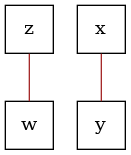
Now, we will show the output given a real CI test, which performs CI hypothesis testing to determine CI in the data. Due to finite data and the presence of noise, there is always a possibility that the CI test makes a mistake.

pc = PC(ci_estimator=ci_estimator)
pc.learn_graph(data, context)

# The resulting completely partially directed acyclic graph (CPDAG) that is learned
# is a "Markov equivalence class", which encodes all the conditional dependences that
# were learned from the data. Note here, because the CI test fails to find the
# dependency between 'z' and 'y', then we fail to also orient the corresponding
# collider in the data. This illustrates the dependency of constraint-based
# structure learning algorithms on the implicit Type I/II error in hypothesis tests.
graph = pc.graph_

dot_graph = draw(graph)
dot_graph.render(outfile="ci_cpdag.png", view=True)

'ci_cpdag.png'