Demo for the DoWhy causal API

We show a simple example of adding a causal extension to any dataframe.

import dowhy.datasets
import dowhy.api

import numpy as np
import pandas as pd

from statsmodels.api import OLS

data = dowhy.datasets.linear_dataset(beta=5,
        num_common_causes=1,
        num_instruments = 0,
        num_samples=1000,
        treatment_is_binary=True)
df = data['df']
df['y'] = df['y'] + np.random.normal(size=len(df)) # Adding noise to data. Without noise, the variance in Y|X, Z is zero, and mcmc fails.
#data['dot_graph'] = 'digraph { v ->y;X0-> v;X0-> y;}'

treatment= data["treatment_name"][0]
outcome = data["outcome_name"][0]
common_cause = data["common_causes_names"][0]
df

	W0	v0	y
0	0.615341	False	-0.216582
1	1.547448	True	3.791882
2	-1.220144	True	4.319986
3	-0.167506	True	6.049082
4	2.950866	True	4.455041
...	...	...	...
995	0.978907	True	6.964400
996	2.768105	True	4.851054
997	0.657292	True	7.053682
998	0.462598	False	0.075282
999	0.544589	True	3.206106

1000 rows × 3 columns

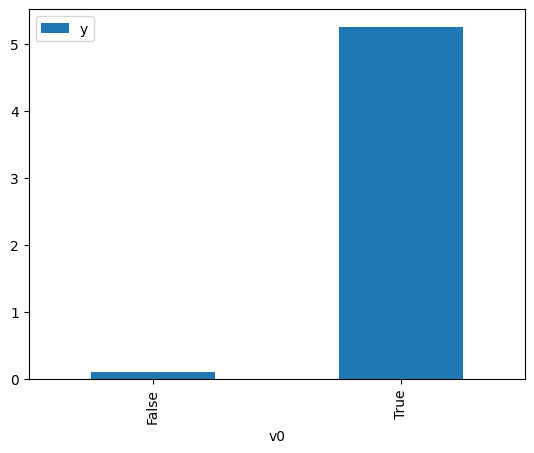
# data['df'] is just a regular pandas.DataFrame
df.causal.do(x=treatment,
                     variable_types={treatment: 'b', outcome: 'c', common_cause: 'c'},
                     outcome=outcome,
                     common_causes=[common_cause],
                     proceed_when_unidentifiable=True).groupby(treatment).mean().plot(y=outcome, kind='bar')

<AxesSubplot: xlabel='v0'>

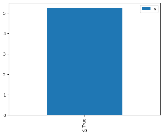
df.causal.do(x={treatment: 1},
              variable_types={treatment:'b', outcome: 'c', common_cause: 'c'},
              outcome=outcome,
              method='weighting',
              common_causes=[common_cause],
              proceed_when_unidentifiable=True).groupby(treatment).mean().plot(y=outcome, kind='bar')

<AxesSubplot: xlabel='v0'>

cdf_1 = df.causal.do(x={treatment: 1},
              variable_types={treatment: 'b', outcome: 'c', common_cause: 'c'},
              outcome=outcome,
              dot_graph=data['dot_graph'],
              proceed_when_unidentifiable=True)

cdf_0 = df.causal.do(x={treatment: 0},
              variable_types={treatment: 'b', outcome: 'c', common_cause: 'c'},
              outcome=outcome,
              dot_graph=data['dot_graph'],
              proceed_when_unidentifiable=True)

cdf_0

	W0	v0	y	propensity_score	weight
0	0.067560	False	1.911379	0.466482	2.143707
1	0.823216	False	-1.139482	0.298868	3.345962
2	1.662468	False	0.487500	0.161029	6.210075
3	1.219407	False	-0.734138	0.226293	4.419058
4	3.170608	False	0.352740	0.043754	22.854844
...	...	...	...	...	...
995	2.290390	False	0.137876	0.095559	10.464770
996	1.037646	False	0.709049	0.257967	3.876460
997	-0.134015	False	1.177118	0.514338	1.944246
998	0.438583	False	-2.028024	0.380597	2.627451
999	-0.018765	False	-1.847223	0.486952	2.053589

1000 rows × 5 columns

cdf_1

	W0	v0	y	propensity_score	weight
0	0.151752	True	5.144520	0.553375	1.807092
1	-0.361275	True	5.457729	0.432065	2.314466
2	-0.516995	True	4.685548	0.396163	2.524211
3	-0.151791	True	7.376667	0.481441	2.077096
4	0.533555	True	4.762663	0.640448	1.561408
...	...	...	...	...	...
995	2.328699	True	5.015506	0.907543	1.101876
996	0.922553	True	6.789926	0.720539	1.387849
997	0.890339	True	5.813846	0.714331	1.399912
998	-0.380071	True	4.574668	0.427686	2.338166
999	1.219794	True	3.804645	0.773772	1.292371

1000 rows × 5 columns

Comparing the estimate to Linear Regression

First, estimating the effect using the causal data frame, and the 95% confidence interval.

(cdf_1['y'] - cdf_0['y']).mean()

$\displaystyle 5.18094679145088$

1.96*(cdf_1['y'] - cdf_0['y']).std() / np.sqrt(len(df))

$\displaystyle 0.0932881847772126$

Comparing to the estimate from OLS.

model = OLS(np.asarray(df[outcome]), np.asarray(df[[common_cause, treatment]], dtype=np.float64))
result = model.fit()
result.summary()

OLS Regression Results

Dep. Variable:	y	R-squared (uncentered):	0.945
Model:	OLS	Adj. R-squared (uncentered):	0.945
Method:	Least Squares	F-statistic:	8643.
Date:	Tue, 06 Dec 2022	Prob (F-statistic):	0.00
Time:	09:38:55	Log-Likelihood:	-1450.1
No. Observations:	1000	AIC:	2904.
Df Residuals:	998	BIC:	2914.
Df Model:	2
Covariance Type:	nonrobust

	coef	std err	t	P>|t|	[0.025	0.975]
x1	0.2364	0.035	6.773	0.000	0.168	0.305
x2	5.0849	0.053	95.597	0.000	4.981	5.189

Omnibus:	0.226	Durbin-Watson:	1.922
Prob(Omnibus):	0.893	Jarque-Bera (JB):	0.264
Skew:	0.035	Prob(JB):	0.876
Kurtosis:	2.962	Cond. No.	2.46

Notes:
[1] R² is computed without centering (uncentered) since the model does not contain a constant.
[2] Standard Errors assume that the covariance matrix of the errors is correctly specified.