Conditional Average Treatment Effects (CATE) with DoWhy and EconML
This is an experimental feature where we use EconML methods from DoWhy. Using EconML allows CATE estimation using different methods.
All four steps of causal inference in DoWhy remain the same: model, identify, estimate, and refute. The key difference is that we now call econml methods in the estimation step. There is also a simpler example using linear regression to understand the intuition behind CATE estimators.
All datasets are generated using linear structural equations.
[1]:
%load_ext autoreload
%autoreload 2
[2]:
import numpy as np
import pandas as pd
import logging

import dowhy
from dowhy import CausalModel
import dowhy.datasets

import econml
import warnings
warnings.filterwarnings('ignore')

BETA = 10
[3]:
data = dowhy.datasets.linear_dataset(BETA, num_common_causes=4, num_samples=10000,
                                    num_instruments=2, num_effect_modifiers=2,
                                     num_treatments=1,
                                    treatment_is_binary=False,
                                    num_discrete_common_causes=2,
                                    num_discrete_effect_modifiers=0,
                                    one_hot_encode=False)
df=data['df']
print(df.head())
print("True causal estimate is", data["ate"])
         X0        X1   Z0        Z1        W0        W1 W2 W3         v0  \
0 -1.139678  0.376798  1.0  0.481657 -1.976460 -1.565492  1  2  14.424988
1 -1.487004 -0.866999  1.0  0.891529 -1.656043  0.601124  3  0  15.535243
2 -2.846174 -0.411779  1.0  0.505546 -0.921121 -0.498449  1  0  12.147642
3 -1.810018  0.505204  1.0  0.584927 -0.377332 -0.025346  1  2  28.093158
4 -0.260961 -0.083155  1.0  0.635962 -0.898638 -0.474116  3  0  14.734871

            y
0   94.606721
1   25.284846
2  -24.335424
3  141.068777
4  126.713651
True causal estimate is 3.859817328248521
[4]:
model = CausalModel(data=data["df"],
                    treatment=data["treatment_name"], outcome=data["outcome_name"],
                    graph=data["gml_graph"])
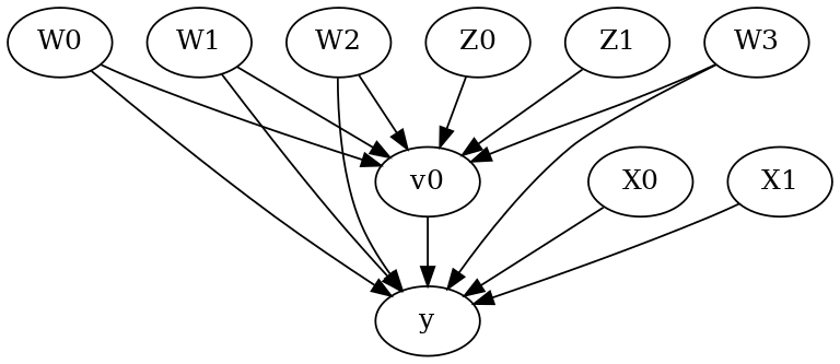
[5]:
model.view_model()
from IPython.display import Image, display
display(Image(filename="causal_model.png"))
[6]:
identified_estimand= model.identify_effect(proceed_when_unidentifiable=True)
print(identified_estimand)
Estimand type: EstimandType.NONPARAMETRIC_ATE

### Estimand : 1
Estimand name: backdoor
Estimand expression:
  d
─────(E[y|W3,W1,W2,W0])
d[v₀]
Estimand assumption 1, Unconfoundedness: If U→{v0} and U→y then P(y|v0,W3,W1,W2,W0,U) = P(y|v0,W3,W1,W2,W0)

### Estimand : 2
Estimand name: iv
Estimand expression:
 ⎡                              -1⎤
 ⎢    d        ⎛    d          ⎞  ⎥
E⎢─────────(y)⋅⎜─────────([v₀])⎟  ⎥
 ⎣d[Z₁  Z₀]    ⎝d[Z₁  Z₀]      ⎠  ⎦
Estimand assumption 1, As-if-random: If U→→y then ¬(U →→{Z1,Z0})
Estimand assumption 2, Exclusion: If we remove {Z1,Z0}→{v0}, then ¬({Z1,Z0}→y)

### Estimand : 3
Estimand name: frontdoor
No such variable(s) found!
Linear Model
First, let us build some intuition using a linear model for estimating CATE. The effect modifiers (that lead to a heterogeneous treatment effect) can be modeled as interaction terms with the treatment. Thus, their value modulates the effect of treatment.
Below the estimated effect of changing treatment from 0 to 1.
[7]:
linear_estimate = model.estimate_effect(identified_estimand,
                                        method_name="backdoor.linear_regression",
                                       control_value=0,
                                       treatment_value=1)
print(linear_estimate)
*** Causal Estimate ***

## Identified estimand
Estimand type: EstimandType.NONPARAMETRIC_ATE

### Estimand : 1
Estimand name: backdoor
Estimand expression:
  d
─────(E[y|W3,W1,W2,W0])
d[v₀]
Estimand assumption 1, Unconfoundedness: If U→{v0} and U→y then P(y|v0,W3,W1,W2,W0,U) = P(y|v0,W3,W1,W2,W0)

## Realized estimand
b: y~v0+W3+W1+W2+W0+v0*X1+v0*X0
Target units: ate

## Estimate
Mean value: 3.860007413016712
EconML methods
We now move to the more advanced methods from the EconML package for estimating CATE.
First, let us look at the double machine learning estimator. Method_name corresponds to the fully qualified name of the class that we want to use. For double ML, it is “econml.dml.DML”.
Target units defines the units over which the causal estimate is to be computed. This can be a lambda function filter on the original dataframe, a new Pandas dataframe, or a string corresponding to the three main kinds of target units (“ate”, “att” and “atc”). Below we show an example of a lambda function.
Method_params are passed directly to EconML. For details on allowed parameters, refer to the EconML documentation.
[8]:
from sklearn.preprocessing import PolynomialFeatures
from sklearn.linear_model import LassoCV
from sklearn.ensemble import GradientBoostingRegressor
dml_estimate = model.estimate_effect(identified_estimand, method_name="backdoor.econml.dml.DML",
                                     control_value = 0,
                                     treatment_value = 1,
                                 target_units = lambda df: df["X0"]>1,  # condition used for CATE
                                 confidence_intervals=False,
                                method_params={"init_params":{'model_y':GradientBoostingRegressor(),
                                                              'model_t': GradientBoostingRegressor(),
                                                              "model_final":LassoCV(fit_intercept=False),
                                                              'featurizer':PolynomialFeatures(degree=1, include_bias=False)},
                                               "fit_params":{}})
print(dml_estimate)
*** Causal Estimate ***

## Identified estimand
Estimand type: EstimandType.NONPARAMETRIC_ATE

### Estimand : 1
Estimand name: backdoor
Estimand expression:
  d
─────(E[y|W3,W1,W2,W0])
d[v₀]
Estimand assumption 1, Unconfoundedness: If U→{v0} and U→y then P(y|v0,W3,W1,W2,W0,U) = P(y|v0,W3,W1,W2,W0)

## Realized estimand
b: y~v0+W3+W1+W2+W0 | X1,X0
Target units: Data subset defined by a function

## Estimate
Mean value: 12.720436965995988
Effect estimates: [[11.92302099]
 [12.34331302]
 [10.01846489]
 [10.46438894]
 [18.09201303]
 [13.93860441]
 [ 8.87936875]
 [14.51166189]
 [ 7.86731183]
 [10.5322804 ]
 [16.34289323]
 [10.87071427]
 [11.8050526 ]
 [24.17451045]
 [12.06723651]
 [ 9.48024167]
 [ 5.11248715]
 [10.10558891]
 [13.24255223]
 [ 9.40723886]
 [13.12887017]
 [13.60104903]
 [ 7.82838681]
 [15.70700713]
 [13.18430119]
 [ 6.11455904]
 [14.91950188]
 [ 9.24326621]
 [13.89586403]
 [14.20779895]
 [11.04572236]
 [16.77602006]
 [10.32611199]
 [13.86876196]
 [16.49682303]
 [10.73687275]
 [ 9.47703761]
 [13.28564959]
 [14.4780372 ]
 [14.05906891]
 [19.04947439]
 [ 8.41255444]
 [12.02321766]
 [16.16962375]
 [ 6.82068211]
 [14.55241295]
 [15.84340217]
 [16.54277034]
 [11.85799198]
 [10.02780566]
 [13.2229851 ]
 [ 9.90826969]
 [11.96377167]
 [13.99802015]
 [18.07261979]
 [10.97178281]
 [10.26844518]
 [11.38563248]
 [11.40068146]
 [12.6893542 ]
 [16.08488764]
 [ 6.98601806]
 [15.78655967]
 [11.97350549]
 [13.28962327]
 [ 9.26583004]
 [ 8.54951546]
 [13.74481038]
 [ 7.2314779 ]
 [13.44979427]
 [21.05223747]
 [ 8.9578681 ]
 [ 5.76982685]
 [13.92358759]
 [18.34429228]
 [ 9.88569861]
 [ 9.3791081 ]
 [17.03001195]
 [15.98454566]
 [ 6.34137174]
 [12.26705381]
 [16.24405213]
 [12.93647653]
 [ 8.94812793]
 [ 9.80060742]
 [18.3755818 ]
 [ 8.96459921]
 [ 8.80545502]
 [10.21440279]
 [ 9.61621914]
 [11.14317349]
 [11.6143174 ]
 [12.17319691]
 [11.04047164]
 [10.00661205]
 [ 7.57555985]
 [14.18607642]
 [13.05334272]
 [16.91306068]
 [15.55896701]
 [13.42697356]
 [11.65583951]
 [10.39029581]
 [14.79440127]
 [15.03920683]
 [17.19272248]
 [11.35847689]
 [14.94793652]
 [15.03109628]
 [15.38323972]
 [16.00367808]
 [13.39271938]
 [20.66076393]
 [10.46187217]
 [11.23426787]
 [13.08611653]
 [15.6028621 ]
 [ 9.09783163]
 [16.50679849]
 [13.87741848]
 [10.72837223]
 [ 6.03736651]
 [15.35980648]
 [10.42837973]
 [13.07306284]
 [10.86193537]
 [17.18923234]
 [15.22458149]
 [14.56443863]
 [ 8.88734489]
 [ 7.35037942]
 [11.55939441]
 [ 7.31010328]
 [13.47435897]
 [13.82136224]
 [13.02519494]
 [ 9.37300894]
 [11.862749  ]
 [12.13527661]
 [20.77513595]
 [ 8.00074512]
 [16.29613057]
 [18.53784172]
 [13.73910008]
 [12.76606689]
 [16.61483899]
 [11.80411062]
 [ 9.51415925]
 [ 8.47784979]
 [ 8.67402654]
 [11.16957468]
 [ 8.03513007]
 [20.15327427]
 [16.07365097]
 [ 8.795085  ]
 [15.65337556]
 [12.20126353]
 [11.33345301]
 [11.25141437]
 [12.03522563]
 [22.12348227]
 [14.02916244]
 [17.93717427]
 [18.75055644]
 [14.86592622]
 [11.2728034 ]
 [10.05972012]
 [13.15345114]
 [13.38300601]
 [14.91158053]
 [16.16491043]
 [10.15840858]
 [14.27335911]
 [16.6680081 ]
 [11.69977664]
 [ 8.0881425 ]
 [ 7.9133902 ]
 [ 7.59764105]
 [17.20941694]
 [12.48933413]
 [14.12048363]
 [14.54096596]
 [13.72298311]
 [19.81727203]
 [14.07989478]
 [16.39078841]
 [16.24143748]
 [ 8.05923335]
 [10.82741413]
 [11.82554572]
 [13.00718038]
 [11.86157096]
 [15.55803236]
 [11.66647842]
 [15.72491899]
 [10.79408047]
 [17.849043  ]
 [12.88556014]
 [13.09483259]
 [12.05979807]
 [14.94866961]
 [17.12568434]
 [15.13369552]
 [13.53999116]
 [12.60593594]
 [11.07158533]
 [ 7.83530467]
 [12.34181136]
 [12.58098018]
 [12.94456403]
 [15.630964  ]
 [11.85062423]
 [15.65443508]
 [10.08739377]
 [12.54860413]
 [10.73415157]
 [ 9.30830078]
 [14.23740119]
 [12.45997117]
 [10.33304844]
 [14.69164143]
 [12.35363804]
 [16.15294025]
 [12.56638804]
 [ 9.32320857]
 [ 9.97512746]
 [ 8.61324844]
 [16.03989971]
 [ 8.60093119]
 [12.60978402]
 [10.85953301]
 [10.07429526]
 [12.42984461]
 [12.70119298]
 [11.5154313 ]
 [17.41686031]
 [14.33110006]
 [12.18275101]
 [ 9.90040049]
 [15.12522591]
 [11.01366744]
 [17.29075725]
 [10.92704005]]
[9]:
print("True causal estimate is", data["ate"])
True causal estimate is 3.859817328248521
[10]:
dml_estimate = model.estimate_effect(identified_estimand, method_name="backdoor.econml.dml.DML",
                                     control_value = 0,
                                     treatment_value = 1,
                                 target_units = 1,  # condition used for CATE
                                 confidence_intervals=False,
                                method_params={"init_params":{'model_y':GradientBoostingRegressor(),
                                                              'model_t': GradientBoostingRegressor(),
                                                              "model_final":LassoCV(fit_intercept=False),
                                                              'featurizer':PolynomialFeatures(degree=1, include_bias=True)},
                                               "fit_params":{}})
print(dml_estimate)
*** Causal Estimate ***

## Identified estimand
Estimand type: EstimandType.NONPARAMETRIC_ATE

### Estimand : 1
Estimand name: backdoor
Estimand expression:
  d
─────(E[y|W3,W1,W2,W0])
d[v₀]
Estimand assumption 1, Unconfoundedness: If U→{v0} and U→y then P(y|v0,W3,W1,W2,W0,U) = P(y|v0,W3,W1,W2,W0)

## Realized estimand
b: y~v0+W3+W1+W2+W0 | X1,X0
Target units:

## Estimate
Mean value: 3.969326578729081
Effect estimates: [[ 7.29582086]
 [ 1.92815734]
 [-1.99117563]
 ...
 [13.32252088]
 [ 2.35166761]
 [-5.98717298]]
CATE Object and Confidence Intervals
EconML provides its own methods to compute confidence intervals. Using BootstrapInference in the example below.
[11]:
from sklearn.preprocessing import PolynomialFeatures
from sklearn.linear_model import LassoCV
from sklearn.ensemble import GradientBoostingRegressor
from econml.inference import BootstrapInference
dml_estimate = model.estimate_effect(identified_estimand,
                                     method_name="backdoor.econml.dml.DML",
                                     target_units = "ate",
                                     confidence_intervals=True,
                                     method_params={"init_params":{'model_y':GradientBoostingRegressor(),
                                                              'model_t': GradientBoostingRegressor(),
                                                              "model_final": LassoCV(fit_intercept=False),
                                                              'featurizer':PolynomialFeatures(degree=1, include_bias=True)},
                                               "fit_params":{
                                                               'inference': BootstrapInference(n_bootstrap_samples=100, n_jobs=-1),
                                                            }
                                              })
print(dml_estimate)
*** Causal Estimate ***

## Identified estimand
Estimand type: EstimandType.NONPARAMETRIC_ATE

### Estimand : 1
Estimand name: backdoor
Estimand expression:
  d
─────(E[y|W3,W1,W2,W0])
d[v₀]
Estimand assumption 1, Unconfoundedness: If U→{v0} and U→y then P(y|v0,W3,W1,W2,W0,U) = P(y|v0,W3,W1,W2,W0)

## Realized estimand
b: y~v0+W3+W1+W2+W0 | X1,X0
Target units: ate

## Estimate
Mean value: 4.018591979356649
Effect estimates: [[ 7.2973789 ]
 [ 1.95906891]
 [-2.02495275]
 ...
 [13.35051274]
 [ 2.37250833]
 [-5.93917981]]
Can provide a new inputs as target units and estimate CATE on them.
[12]:
test_cols= data['effect_modifier_names'] # only need effect modifiers' values
test_arr = [np.random.uniform(0,1, 10) for _ in range(len(test_cols))] # all variables are sampled uniformly, sample of 10
test_df = pd.DataFrame(np.array(test_arr).transpose(), columns=test_cols)
dml_estimate = model.estimate_effect(identified_estimand,
                                     method_name="backdoor.econml.dml.DML",
                                     target_units = test_df,
                                     confidence_intervals=False,
                                     method_params={"init_params":{'model_y':GradientBoostingRegressor(),
                                                              'model_t': GradientBoostingRegressor(),
                                                              "model_final":LassoCV(),
                                                              'featurizer':PolynomialFeatures(degree=1, include_bias=True)},
                                               "fit_params":{}
                                              })
print(dml_estimate.cate_estimates)
[[14.60220855]
 [16.1024444 ]
 [13.80220789]
 [15.15581876]
 [14.15690416]
 [16.14399702]
 [13.30103866]
 [16.03904845]
 [13.59361577]
 [15.05822401]]
Can also retrieve the raw EconML estimator object for any further operations
[13]:
print(dml_estimate._estimator_object)
<econml.dml.dml.DML object at 0x7fbbe9be8070>
Works with any EconML method
In addition to double machine learning, below we example analyses using orthogonal forests, DRLearner (bug to fix), and neural network-based instrumental variables.
Binary treatment, Binary outcome
[14]:
data_binary = dowhy.datasets.linear_dataset(BETA, num_common_causes=4, num_samples=10000,
                                    num_instruments=2, num_effect_modifiers=2,
                                    treatment_is_binary=True, outcome_is_binary=True)
# convert boolean values to {0,1} numeric
data_binary['df'].v0 = data_binary['df'].v0.astype(int)
data_binary['df'].y = data_binary['df'].y.astype(int)
print(data_binary['df'])

model_binary = CausalModel(data=data_binary["df"],
                    treatment=data_binary["treatment_name"], outcome=data_binary["outcome_name"],
                    graph=data_binary["gml_graph"])
identified_estimand_binary = model_binary.identify_effect(proceed_when_unidentifiable=True)
            X0        X1   Z0        Z1        W0        W1        W2  \
0    -1.031666 -0.676004  0.0  0.048095  0.304211  1.057433  0.753802
1    -0.723289  1.211224  0.0  0.429334  1.689972 -0.065898 -0.420588
2    -0.111164  0.964640  0.0  0.192904 -0.293054  1.326678 -1.338993
3     0.717750  1.585226  0.0  0.178885  0.977203 -1.212051  0.851419
4    -0.047097  2.195409  0.0  0.325146  1.593862 -0.800925 -0.575807
...        ...       ...  ...       ...       ...       ...       ...
9995 -0.006959 -1.434996  0.0  0.814772  1.928532  0.488331 -1.356220
9996  0.868295 -0.215757  0.0  0.011453 -0.319300 -1.272306 -0.257379
9997  1.455640  1.544373  0.0  0.228082 -0.168873  0.001067 -0.533737
9998  0.275809 -0.012997  0.0  0.832838 -1.168387  0.047412 -0.926547
9999  0.228798  1.629531  0.0  0.657545  2.415097 -1.906546  0.857451

            W3  v0  y
0     1.056604   1  1
1     1.492395   1  1
2     0.597437   1  1
3    -1.248664   1  1
4    -0.113636   1  1
...        ...  .. ..
9995  0.724706   1  1
9996 -0.124601   0  0
9997  0.831595   1  1
9998  1.534769   1  1
9999 -1.092122   1  1

[10000 rows x 10 columns]
Using DRLearner estimator
[15]:
from sklearn.linear_model import LogisticRegressionCV
#todo needs binary y
drlearner_estimate = model_binary.estimate_effect(identified_estimand_binary,
                                method_name="backdoor.econml.dr.LinearDRLearner",
                                confidence_intervals=False,
                                method_params={"init_params":{
                                                    'model_propensity': LogisticRegressionCV(cv=3, solver='lbfgs', multi_class='auto')
                                                    },
                                               "fit_params":{}
                                              })
print(drlearner_estimate)
print("True causal estimate is", data_binary["ate"])
*** Causal Estimate ***

## Identified estimand
Estimand type: EstimandType.NONPARAMETRIC_ATE

### Estimand : 1
Estimand name: backdoor
Estimand expression:
  d
─────(E[y|W3,W1,W2,W0])
d[v₀]
Estimand assumption 1, Unconfoundedness: If U→{v0} and U→y then P(y|v0,W3,W1,W2,W0,U) = P(y|v0,W3,W1,W2,W0)

## Realized estimand
b: y~v0+W3+W1+W2+W0 | X1,X0
Target units: ate

## Estimate
Mean value: 0.7844719745032825
Effect estimates: [[0.62888753]
 [0.74144192]
 [0.7598003 ]
 ...
 [0.86898065]
 [0.72920186]
 [0.81117764]]

True causal estimate is 0.6291
Instrumental Variable Method
[16]:
import keras
dims_zx = len(model.get_instruments())+len(model.get_effect_modifiers())
dims_tx = len(model._treatment)+len(model.get_effect_modifiers())
treatment_model = keras.Sequential([keras.layers.Dense(128, activation='relu', input_shape=(dims_zx,)), # sum of dims of Z and X
                                    keras.layers.Dropout(0.17),
                                    keras.layers.Dense(64, activation='relu'),
                                    keras.layers.Dropout(0.17),
                                    keras.layers.Dense(32, activation='relu'),
                                    keras.layers.Dropout(0.17)])
response_model = keras.Sequential([keras.layers.Dense(128, activation='relu', input_shape=(dims_tx,)), # sum of dims of T and X
                                    keras.layers.Dropout(0.17),
                                    keras.layers.Dense(64, activation='relu'),
                                    keras.layers.Dropout(0.17),
                                    keras.layers.Dense(32, activation='relu'),
                                    keras.layers.Dropout(0.17),
                                    keras.layers.Dense(1)])

deepiv_estimate = model.estimate_effect(identified_estimand,
                                        method_name="iv.econml.iv.nnet.DeepIV",
                                        target_units = lambda df: df["X0"]>-1,
                                        confidence_intervals=False,
                                method_params={"init_params":{'n_components': 10, # Number of gaussians in the mixture density networks
                                                              'm': lambda z, x: treatment_model(keras.layers.concatenate([z, x])), # Treatment model,
                                                              "h": lambda t, x: response_model(keras.layers.concatenate([t, x])), # Response model
                                                              'n_samples': 1, # Number of samples used to estimate the response
                                                              'first_stage_options': {'epochs':25},
                                                              'second_stage_options': {'epochs':25}
                                                             },
                                               "fit_params":{}})
print(deepiv_estimate)
2022-12-06 09:31:36.591290: I tensorflow/core/platform/cpu_feature_guard.cc:193] This TensorFlow binary is optimized with oneAPI Deep Neural Network Library (oneDNN) to use the following CPU instructions in performance-critical operations:  AVX2 AVX512F FMA
To enable them in other operations, rebuild TensorFlow with the appropriate compiler flags.
2022-12-06 09:31:36.740590: W tensorflow/compiler/xla/stream_executor/platform/default/dso_loader.cc:64] Could not load dynamic library 'libcudart.so.11.0'; dlerror: libcudart.so.11.0: cannot open shared object file: No such file or directory
2022-12-06 09:31:36.740626: I tensorflow/compiler/xla/stream_executor/cuda/cudart_stub.cc:29] Ignore above cudart dlerror if you do not have a GPU set up on your machine.
2022-12-06 09:31:37.492796: W tensorflow/compiler/xla/stream_executor/platform/default/dso_loader.cc:64] Could not load dynamic library 'libnvinfer.so.7'; dlerror: libnvinfer.so.7: cannot open shared object file: No such file or directory
2022-12-06 09:31:37.492921: W tensorflow/compiler/xla/stream_executor/platform/default/dso_loader.cc:64] Could not load dynamic library 'libnvinfer_plugin.so.7'; dlerror: libnvinfer_plugin.so.7: cannot open shared object file: No such file or directory
2022-12-06 09:31:37.492932: W tensorflow/compiler/tf2tensorrt/utils/py_utils.cc:38] TF-TRT Warning: Cannot dlopen some TensorRT libraries. If you would like to use Nvidia GPU with TensorRT, please make sure the missing libraries mentioned above are installed properly.
2022-12-06 09:31:38.357701: W tensorflow/compiler/xla/stream_executor/platform/default/dso_loader.cc:64] Could not load dynamic library 'libcuda.so.1'; dlerror: libcuda.so.1: cannot open shared object file: No such file or directory
2022-12-06 09:31:38.357734: W tensorflow/compiler/xla/stream_executor/cuda/cuda_driver.cc:265] failed call to cuInit: UNKNOWN ERROR (303)
2022-12-06 09:31:38.357758: I tensorflow/compiler/xla/stream_executor/cuda/cuda_diagnostics.cc:156] kernel driver does not appear to be running on this host (780bf0ca5803): /proc/driver/nvidia/version does not exist
2022-12-06 09:31:38.358307: I tensorflow/core/platform/cpu_feature_guard.cc:193] This TensorFlow binary is optimized with oneAPI Deep Neural Network Library (oneDNN) to use the following CPU instructions in performance-critical operations:  AVX2 AVX512F FMA
To enable them in other operations, rebuild TensorFlow with the appropriate compiler flags.
Epoch 1/25
313/313 [==============================] - 2s 2ms/step - loss: 11.3145
Epoch 2/25
313/313 [==============================] - 0s 2ms/step - loss: 3.7139
Epoch 3/25
313/313 [==============================] - 1s 2ms/step - loss: 3.0487
Epoch 4/25
313/313 [==============================] - 1s 2ms/step - loss: 2.9475
Epoch 5/25
313/313 [==============================] - 0s 1ms/step - loss: 2.8864
Epoch 6/25
313/313 [==============================] - 0s 2ms/step - loss: 2.8635
Epoch 7/25
313/313 [==============================] - 0s 2ms/step - loss: 2.8577
Epoch 8/25
313/313 [==============================] - 0s 1ms/step - loss: 2.8300
Epoch 9/25
313/313 [==============================] - 0s 2ms/step - loss: 2.8035
Epoch 10/25
313/313 [==============================] - 0s 1ms/step - loss: 2.7792
Epoch 11/25
313/313 [==============================] - 0s 1ms/step - loss: 2.7572
Epoch 12/25
313/313 [==============================] - 0s 2ms/step - loss: 2.7487
Epoch 13/25
313/313 [==============================] - 0s 2ms/step - loss: 2.7400
Epoch 14/25
313/313 [==============================] - 0s 1ms/step - loss: 2.7319
Epoch 15/25
313/313 [==============================] - 0s 2ms/step - loss: 2.7320
Epoch 16/25
313/313 [==============================] - 0s 2ms/step - loss: 2.7215
Epoch 17/25
313/313 [==============================] - 0s 1ms/step - loss: 2.7104
Epoch 18/25
313/313 [==============================] - 0s 2ms/step - loss: 2.7143
Epoch 19/25
313/313 [==============================] - 0s 2ms/step - loss: 2.6999
Epoch 20/25
313/313 [==============================] - 0s 2ms/step - loss: 2.7023
Epoch 21/25
313/313 [==============================] - 0s 2ms/step - loss: 2.7044
Epoch 22/25
313/313 [==============================] - 0s 1ms/step - loss: 2.6966
Epoch 23/25
313/313 [==============================] - 0s 2ms/step - loss: 2.6917
Epoch 24/25
313/313 [==============================] - 0s 2ms/step - loss: 2.6949
Epoch 25/25
313/313 [==============================] - 0s 1ms/step - loss: 2.6876
Epoch 1/25
313/313 [==============================] - 2s 2ms/step - loss: 14380.6426
Epoch 2/25
313/313 [==============================] - 1s 2ms/step - loss: 6956.3730
Epoch 3/25
313/313 [==============================] - 1s 2ms/step - loss: 5785.6792
Epoch 4/25
313/313 [==============================] - 1s 2ms/step - loss: 4512.2324
Epoch 5/25
313/313 [==============================] - 1s 2ms/step - loss: 4286.8223
Epoch 6/25
313/313 [==============================] - 1s 2ms/step - loss: 4080.0771
Epoch 7/25
313/313 [==============================] - 1s 2ms/step - loss: 4319.6016
Epoch 8/25
313/313 [==============================] - 1s 2ms/step - loss: 4135.0430
Epoch 9/25
313/313 [==============================] - 1s 2ms/step - loss: 3988.2073
Epoch 10/25
313/313 [==============================] - 1s 2ms/step - loss: 4028.9875
Epoch 11/25
313/313 [==============================] - 1s 2ms/step - loss: 4053.9436
Epoch 12/25
313/313 [==============================] - 1s 2ms/step - loss: 3989.8782
Epoch 13/25
313/313 [==============================] - 1s 2ms/step - loss: 3880.1321
Epoch 14/25
313/313 [==============================] - 1s 2ms/step - loss: 3997.8403
Epoch 15/25
313/313 [==============================] - 1s 2ms/step - loss: 4091.7065
Epoch 16/25
313/313 [==============================] - 1s 2ms/step - loss: 3943.5959
Epoch 17/25
313/313 [==============================] - 1s 2ms/step - loss: 3872.4724
Epoch 18/25
313/313 [==============================] - 1s 2ms/step - loss: 3904.8862
Epoch 19/25
313/313 [==============================] - 1s 2ms/step - loss: 3919.0620
Epoch 20/25
313/313 [==============================] - 1s 2ms/step - loss: 3949.4932
Epoch 21/25
313/313 [==============================] - 1s 2ms/step - loss: 3974.3538
Epoch 22/25
313/313 [==============================] - 1s 2ms/step - loss: 3894.0610
Epoch 23/25
313/313 [==============================] - 1s 2ms/step - loss: 3907.8286
Epoch 24/25
313/313 [==============================] - 1s 2ms/step - loss: 3881.0784
Epoch 25/25
313/313 [==============================] - 1s 2ms/step - loss: 3876.5708
WARNING:tensorflow:
The following Variables were used a Lambda layer's call (lambda_7), but
are not present in its tracked objects:
  <tf.Variable 'dense_3/kernel:0' shape=(3, 128) dtype=float32>
  <tf.Variable 'dense_3/bias:0' shape=(128,) dtype=float32>
  <tf.Variable 'dense_4/kernel:0' shape=(128, 64) dtype=float32>
  <tf.Variable 'dense_4/bias:0' shape=(64,) dtype=float32>
  <tf.Variable 'dense_5/kernel:0' shape=(64, 32) dtype=float32>
  <tf.Variable 'dense_5/bias:0' shape=(32,) dtype=float32>
  <tf.Variable 'dense_6/kernel:0' shape=(32, 1) dtype=float32>
  <tf.Variable 'dense_6/bias:0' shape=(1,) dtype=float32>
It is possible that this is intended behavior, but it is more likely
an omission. This is a strong indication that this layer should be
formulated as a subclassed Layer rather than a Lambda layer.
159/159 [==============================] - 0s 765us/step
159/159 [==============================] - 0s 782us/step
*** Causal Estimate ***

## Identified estimand
Estimand type: EstimandType.NONPARAMETRIC_ATE

### Estimand : 1
Estimand name: iv
Estimand expression:
 ⎡                              -1⎤
 ⎢    d        ⎛    d          ⎞  ⎥
E⎢─────────(y)⋅⎜─────────([v₀])⎟  ⎥
 ⎣d[Z₁  Z₀]    ⎝d[Z₁  Z₀]      ⎠  ⎦
Estimand assumption 1, As-if-random: If U→→y then ¬(U →→{Z1,Z0})
Estimand assumption 2, Exclusion: If we remove {Z1,Z0}→{v0}, then ¬({Z1,Z0}→y)

## Realized estimand
b: y~v0+W3+W1+W2+W0 | X1,X0
Target units: Data subset defined by a function

## Estimate
Mean value: 0.6094349026679993
Effect estimates: [[0.39437866]
 [0.54998016]
 [0.88456726]
 ...
 [0.7917938 ]
 [0.366745  ]
 [0.24130249]]
Metalearners
[17]:
data_experiment = dowhy.datasets.linear_dataset(BETA, num_common_causes=5, num_samples=10000,
                                    num_instruments=2, num_effect_modifiers=5,
                                    treatment_is_binary=True, outcome_is_binary=False)
# convert boolean values to {0,1} numeric
data_experiment['df'].v0 = data_experiment['df'].v0.astype(int)
print(data_experiment['df'])
model_experiment = CausalModel(data=data_experiment["df"],
                    treatment=data_experiment["treatment_name"], outcome=data_experiment["outcome_name"],
                    graph=data_experiment["gml_graph"])
identified_estimand_experiment = model_experiment.identify_effect(proceed_when_unidentifiable=True)
            X0        X1        X2        X3        X4   Z0        Z1  \
0    -0.596220  0.099887  0.736421  0.355603  0.380334  1.0  0.300393
1    -0.698411  0.627258 -1.432214 -0.091191  1.465805  1.0  0.247807
2    -0.413890 -1.770966  0.109496  0.765003  1.309041  1.0  0.849533
3     0.987063  0.936157 -1.573284 -0.500667  2.423877  1.0  0.273627
4    -0.452387  1.061270 -0.594140 -0.257712  0.802644  0.0  0.519093
...        ...       ...       ...       ...       ...  ...       ...
9995  0.759189  0.342091 -0.706739 -1.349456  1.089102  1.0  0.356326
9996  2.080483  0.492555 -0.694581 -0.742124  3.178105  1.0  0.377141
9997  2.559396 -0.522164 -1.176900  0.116382  0.897286  1.0  0.348116
9998 -0.808144  0.468375 -1.198330  0.788004 -0.375836  1.0  0.661173
9999  0.359070 -0.071868  0.355890 -1.531252  1.071477  1.0  0.095732

            W0        W1        W2        W3        W4  v0          y
0     2.013239  1.783825 -0.920312  1.848727 -0.802548   1  21.461043
1     0.262221 -0.051600  0.225691 -1.056805  0.097859   1   7.303609
2    -0.426950 -1.195348 -1.002037 -0.609264 -0.571706   1   9.800877
3    -0.794498 -0.302214 -0.972552  0.459671 -0.319626   1   6.115136
4     1.165453  2.589719 -0.308291  1.777965 -1.311154   1  16.044881
...        ...       ...       ...       ...       ...  ..        ...
9995  0.476187  0.848299  0.478442  1.843532 -0.288942   1  10.367019
9996 -1.821473  1.253179  0.629680  1.401768 -1.168365   1  14.424610
9997 -0.162720 -1.234578 -0.291430  0.476172 -0.192130   1   8.182621
9998  0.247771  1.299142  0.972288  0.706067 -1.704687   1   9.979288
9999 -1.492734  1.627237 -0.056593 -0.233981 -0.659690   1   8.589204

[10000 rows x 14 columns]
[18]:
from sklearn.ensemble import RandomForestRegressor
metalearner_estimate = model_experiment.estimate_effect(identified_estimand_experiment,
                                method_name="backdoor.econml.metalearners.TLearner",
                                confidence_intervals=False,
                                method_params={"init_params":{
                                                    'models': RandomForestRegressor()
                                                    },
                                               "fit_params":{}
                                              })
print(metalearner_estimate)
print("True causal estimate is", data_experiment["ate"])
*** Causal Estimate ***

## Identified estimand
Estimand type: EstimandType.NONPARAMETRIC_ATE

### Estimand : 1
Estimand name: backdoor
Estimand expression:
  d
─────(E[y|W3,W1,W4,W2,W0])
d[v₀]
Estimand assumption 1, Unconfoundedness: If U→{v0} and U→y then P(y|v0,W3,W1,W4,W2,W0,U) = P(y|v0,W3,W1,W4,W2,W0)

## Realized estimand
b: y~v0+X3+X0+X1+X2+X4+W3+W1+W4+W2+W0
Target units: ate

## Estimate
Mean value: 13.479294111047254
Effect estimates: [[22.23518159]
 [ 8.18475338]
 [16.230422  ]
 ...
 [12.07270731]
 [10.86509234]
 [11.57870552]]

True causal estimate is 10.983332422616362
Avoiding retraining the estimator
Once an estimator is fitted, it can be reused to estimate effect on different data points. In this case, you can pass fit_estimator=False to estimate_effect. This works for any EconML estimator. We show an example for the T-learner below.
[19]:
# For metalearners, need to provide all the features (except treatmeant and outcome)
metalearner_estimate = model_experiment.estimate_effect(identified_estimand_experiment,
                                method_name="backdoor.econml.metalearners.TLearner",
                                confidence_intervals=False,
                                fit_estimator=False,
                                target_units=data_experiment["df"].drop(["v0","y", "Z0", "Z1"], axis=1)[9995:],
                                method_params={})
print(metalearner_estimate)
print("True causal estimate is", data_experiment["ate"])
*** Causal Estimate ***

## Identified estimand
Estimand type: EstimandType.NONPARAMETRIC_ATE

### Estimand : 1
Estimand name: backdoor
Estimand expression:
  d
─────(E[y|W3,W1,W4,W2,W0])
d[v₀]
Estimand assumption 1, Unconfoundedness: If U→{v0} and U→y then P(y|v0,W3,W1,W4,W2,W0,U) = P(y|v0,W3,W1,W4,W2,W0)

## Realized estimand
b: y~v0+X3+X0+X1+X2+X4+W3+W1+W4+W2+W0
Target units: Data subset provided as a data frame

## Estimate
Mean value: 12.197050885889805
Effect estimates: [[10.6831902 ]
 [15.78555907]
 [12.07270731]
 [10.86509234]
 [11.57870552]]

True causal estimate is 10.983332422616362
Refuting the estimate
Adding a random common cause variable
[20]:
res_random=model.refute_estimate(identified_estimand, dml_estimate, method_name="random_common_cause")
print(res_random)
Refute: Add a random common cause
Estimated effect:14.795550768174639
New effect:14.70451900651505
p value:0.3999999999999999
Adding an unobserved common cause variable
[21]:
res_unobserved=model.refute_estimate(identified_estimand, dml_estimate, method_name="add_unobserved_common_cause",
                                     confounders_effect_on_treatment="linear", confounders_effect_on_outcome="linear",
                                    effect_strength_on_treatment=0.01, effect_strength_on_outcome=0.02)
print(res_unobserved)
Refute: Add an Unobserved Common Cause
Estimated effect:14.795550768174639
New effect:14.837278264989099
Replacing treatment with a random (placebo) variable
[22]:
res_placebo=model.refute_estimate(identified_estimand, dml_estimate,
        method_name="placebo_treatment_refuter", placebo_type="permute",
        num_simulations=10 # at least 100 is good, setting to 10 for speed
        )
print(res_placebo)
Refute: Use a Placebo Treatment
Estimated effect:14.795550768174639
New effect:-0.03871899781084483
p value:0.3852270982452243
Removing a random subset of the data
[23]:
res_subset=model.refute_estimate(identified_estimand, dml_estimate,
        method_name="data_subset_refuter", subset_fraction=0.8,
        num_simulations=10)
print(res_subset)
Refute: Use a subset of data
Estimated effect:14.795550768174639
New effect:14.803899918929867
p value:0.47997676494495317
More refutation methods to come, especially specific to the CATE estimators.