Estimating effect of multiple treatments#
[1]:
from dowhy import CausalModel
import dowhy.datasets

import warnings
warnings.filterwarnings('ignore')
[2]:
data = dowhy.datasets.linear_dataset(10, num_common_causes=4, num_samples=10000,
                                     num_instruments=0, num_effect_modifiers=2,
                                     num_treatments=2,
                                     treatment_is_binary=False,
                                     num_discrete_common_causes=2,
                                     num_discrete_effect_modifiers=0,
                                     one_hot_encode=False)
df=data['df']
df.head()
[2]:
| X0 | X1 | W0 | W1 | W2 | W3 | v0 | v1 | y | |
|---|---|---|---|---|---|---|---|---|---|
| 0 | 1.893067 | 0.103583 | 0.048774 | 0.972218 | 1 | 2 | 13.820447 | 9.255445 | 1131.823214 |
| 1 | 0.513345 | 2.809553 | -0.298139 | 0.897915 | 3 | 2 | 14.397815 | 13.311720 | 745.836325 |
| 2 | 0.059413 | 0.054502 | -0.088567 | -0.197696 | 0 | 2 | 8.459518 | -2.017247 | 62.606043 |
| 3 | 1.159260 | 2.128179 | -1.251880 | -0.968904 | 0 | 1 | 0.005658 | -5.655181 | -60.851593 |
| 4 | 1.306482 | 0.121526 | -1.995050 | -0.678983 | 3 | 1 | 1.250531 | 1.173030 | 36.743750 |
[3]:
model = CausalModel(data=data["df"],
                    treatment=data["treatment_name"], outcome=data["outcome_name"],
                    graph=data["gml_graph"])
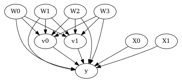
[4]:
model.view_model()
from IPython.display import Image, display
display(Image(filename="causal_model.png"))
[5]:
identified_estimand= model.identify_effect(proceed_when_unidentifiable=True)
print(identified_estimand)
Estimand type: EstimandType.NONPARAMETRIC_ATE

### Estimand : 1
Estimand name: backdoor
Estimand expression:
    d
─────────(E[y|W1,W2,W0,W3])
d[v₀  v₁]
Estimand assumption 1, Unconfoundedness: If U→{v0,v1} and U→y then P(y|v0,v1,W1,W2,W0,W3,U) = P(y|v0,v1,W1,W2,W0,W3)

### Estimand : 2
Estimand name: iv
No such variable(s) found!

### Estimand : 3
Estimand name: frontdoor
No such variable(s) found!
Linear model#
Let us first see an example for a linear model. The control_value and treatment_value can be provided as a tuple/list when the treatment is multi-dimensional.
The interpretation is change in y when v0 and v1 are changed from (0,0) to (1,1).
[6]:
linear_estimate = model.estimate_effect(identified_estimand,
                                        method_name="backdoor.linear_regression",
                                        control_value=(0,0),
                                        treatment_value=(1,1),
                                        method_params={'need_conditional_estimates': False})
print(linear_estimate)
*** Causal Estimate ***

## Identified estimand
Estimand type: EstimandType.NONPARAMETRIC_ATE

### Estimand : 1
Estimand name: backdoor
Estimand expression:
    d
─────────(E[y|W1,W2,W0,W3])
d[v₀  v₁]
Estimand assumption 1, Unconfoundedness: If U→{v0,v1} and U→y then P(y|v0,v1,W1,W2,W0,W3,U) = P(y|v0,v1,W1,W2,W0,W3)

## Realized estimand
b: y~v0+v1+W1+W2+W0+W3+v0*X0+v0*X1+v1*X0+v1*X1
Target units: ate

## Estimate
Mean value: 49.86459109879479
You can estimate conditional effects, based on effect modifiers.
[7]:
linear_estimate = model.estimate_effect(identified_estimand,
                                        method_name="backdoor.linear_regression",
                                        control_value=(0,0),
                                        treatment_value=(1,1))
print(linear_estimate)
*** Causal Estimate ***

## Identified estimand
Estimand type: EstimandType.NONPARAMETRIC_ATE

### Estimand : 1
Estimand name: backdoor
Estimand expression:
    d
─────────(E[y|W1,W2,W0,W3])
d[v₀  v₁]
Estimand assumption 1, Unconfoundedness: If U→{v0,v1} and U→y then P(y|v0,v1,W1,W2,W0,W3,U) = P(y|v0,v1,W1,W2,W0,W3)

## Realized estimand
b: y~v0+v1+W1+W2+W0+W3+v0*X0+v0*X1+v1*X0+v1*X1
Target units:

## Estimate
Mean value: 49.86459109879479
### Conditional Estimates
__categorical__X0  __categorical__X1
(-3.252, -0.0735]  (-3.1799999999999997, -0.296]     -5.959011
                   (-0.296, 0.302]                   -3.445913
                   (0.302, 0.826]                    -3.262347
                   (0.826, 1.409]                    -4.914089
                   (1.409, 4.772]                    -1.098686
(-0.0735, 0.52]    (-3.1799999999999997, -0.296]     27.392269
                   (-0.296, 0.302]                   28.838159
                   (0.302, 0.826]                    30.072040
                   (0.826, 1.409]                    30.641640
                   (1.409, 4.772]                    32.283592
(0.52, 1.029]      (-3.1799999999999997, -0.296]     48.168435
                   (-0.296, 0.302]                   49.191962
                   (0.302, 0.826]                    49.943283
                   (0.826, 1.409]                    51.100576
                   (1.409, 4.772]                    52.287870
(1.029, 1.599]     (-3.1799999999999997, -0.296]     68.254575
                   (-0.296, 0.302]                   69.782471
                   (0.302, 0.826]                    70.859518
                   (0.826, 1.409]                    70.892093
                   (1.409, 4.772]                    72.500243
(1.599, 4.389]     (-3.1799999999999997, -0.296]    100.358743
                   (-0.296, 0.302]                  102.224670
                   (0.302, 0.826]                   103.162188
                   (0.826, 1.409]                   102.369651
                   (1.409, 4.772]                   104.967850
dtype: float64
More methods#
You can also use methods from EconML or CausalML libraries that support multiple treatments. You can look at examples from the conditional effect notebook: https://py-why.github.io/dowhy/example_notebooks/dowhy-conditional-treatment-effects.html
Propensity-based methods do not support multiple treatments currently.