DoWhy: Interpreters for Causal Estimators#
This is a quick introduction to the use of interpreters in the DoWhy causal inference library. We will load in a sample dataset, use different methods for estimating the causal effect of a (pre-specified)treatment variable on a (pre-specified) outcome variable and demonstrate how to interpret the obtained results.
First, let us add the required path for Python to find the DoWhy code and load all required packages
[1]:
%load_ext autoreload
%autoreload 2
[2]:
import numpy as np
import pandas as pd
import logging

import dowhy
from dowhy import CausalModel
import dowhy.datasets
Now, let us load a dataset. For simplicity, we simulate a dataset with linear relationships between common causes and treatment, and common causes and outcome.
Beta is the true causal effect.
[3]:
data = dowhy.datasets.linear_dataset(beta=1,
        num_common_causes=5,
        num_instruments = 2,
        num_treatments=1,
        num_discrete_common_causes=1,
        num_samples=10000,
        treatment_is_binary=True,
        outcome_is_binary=False)
df = data["df"]
print(df[df.v0==True].shape[0])
df
7636
[3]:
| Z0 | Z1 | W0 | W1 | W2 | W3 | W4 | v0 | y | |
|---|---|---|---|---|---|---|---|---|---|
| 0 | 1.0 | 0.910918 | 0.112709 | 1.690538 | -1.254488 | -1.445755 | 2 | True | 1.262203 |
| 1 | 0.0 | 0.318279 | -0.119906 | 0.562458 | 0.405494 | -0.144709 | 0 | True | 1.623785 |
| 2 | 0.0 | 0.272863 | -0.250231 | 1.766001 | -0.834673 | -0.276058 | 1 | True | 1.854648 |
| 3 | 1.0 | 0.949554 | 0.546074 | 0.410488 | -2.021715 | 1.875669 | 2 | True | 1.193100 |
| 4 | 0.0 | 0.742739 | -0.364563 | -0.852032 | -2.072905 | -0.250494 | 2 | False | -2.191271 |
| ... | ... | ... | ... | ... | ... | ... | ... | ... | ... |
| 9995 | 0.0 | 0.481639 | 0.759033 | 0.330807 | 0.688863 | 0.323130 | 2 | True | 2.271962 |
| 9996 | 1.0 | 0.106936 | -0.838163 | 1.992728 | 0.123482 | 0.692196 | 1 | True | 2.766560 |
| 9997 | 1.0 | 0.979827 | -0.087278 | -0.379637 | -0.642882 | -0.378059 | 2 | True | 0.175837 |
| 9998 | 0.0 | 0.428467 | -1.284235 | 1.441514 | 1.267610 | 2.458900 | 3 | True | 3.624072 |
| 9999 | 0.0 | 0.537643 | 0.069879 | 1.470142 | 1.034044 | 1.390796 | 0 | False | 2.525064 |
10000 rows × 9 columns
Note that we are using a pandas dataframe to load the data.
Identifying the causal estimand#
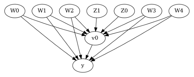
We now input a causal graph in the GML graph format.
[4]:
# With graph
model=CausalModel(
        data = df,
        treatment=data["treatment_name"],
        outcome=data["outcome_name"],
        graph=data["gml_graph"],
        instruments=data["instrument_names"]
        )
[5]:
model.view_model()
[6]:
from IPython.display import Image, display
display(Image(filename="causal_model.png"))
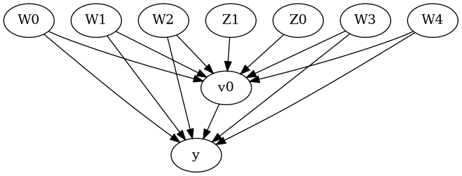
We get a causal graph. Now identification and estimation is done.
[7]:
identified_estimand = model.identify_effect(proceed_when_unidentifiable=True)
print(identified_estimand)
Estimand type: EstimandType.NONPARAMETRIC_ATE

### Estimand : 1
Estimand name: backdoor
Estimand expression:
  d
─────(E[y|W1,W3,W4,W2,W0])
d[v₀]
Estimand assumption 1, Unconfoundedness: If U→{v0} and U→y then P(y|v0,W1,W3,W4,W2,W0,U) = P(y|v0,W1,W3,W4,W2,W0)

### Estimand : 2
Estimand name: iv
Estimand expression:
 ⎡                              -1⎤
 ⎢    d        ⎛    d          ⎞  ⎥
E⎢─────────(y)⋅⎜─────────([v₀])⎟  ⎥
 ⎣d[Z₀  Z₁]    ⎝d[Z₀  Z₁]      ⎠  ⎦
Estimand assumption 1, As-if-random: If U→→y then ¬(U →→{Z0,Z1})
Estimand assumption 2, Exclusion: If we remove {Z0,Z1}→{v0}, then ¬({Z0,Z1}→y)

### Estimand : 3
Estimand name: frontdoor
No such variable(s) found!
Method 1: Propensity Score Stratification#
We will be using propensity scores to stratify units in the data.
[8]:
causal_estimate_strat = model.estimate_effect(identified_estimand,
                                              method_name="backdoor.propensity_score_stratification",
                                              target_units="att")
print(causal_estimate_strat)
print("Causal Estimate is " + str(causal_estimate_strat.value))
*** Causal Estimate ***

## Identified estimand
Estimand type: EstimandType.NONPARAMETRIC_ATE

### Estimand : 1
Estimand name: backdoor
Estimand expression:
  d
─────(E[y|W1,W3,W4,W2,W0])
d[v₀]
Estimand assumption 1, Unconfoundedness: If U→{v0} and U→y then P(y|v0,W1,W3,W4,W2,W0,U) = P(y|v0,W1,W3,W4,W2,W0)

## Realized estimand
b: y~v0+W1+W3+W4+W2+W0
Target units: att

## Estimate
Mean value: 1.0060750804064682

Causal Estimate is 1.0060750804064682
Textual Interpreter#
The textual Interpreter describes (in words) the effect of unit change in the treatment variable on the outcome variable.
[9]:
# Textual Interpreter
interpretation = causal_estimate_strat.interpret(method_name="textual_effect_interpreter")
Increasing the treatment variable(s) [v0] from 0 to 1 causes an increase of 1.0060750804064682 in the expected value of the outcome [['y']], over the data distribution/population represented by the dataset.
Visual Interpreter#
The visual interpreter plots the change in the standardized mean difference (SMD) before and after Propensity Score based adjustment of the dataset. The formula for SMD is given below.
\(SMD = \frac{\bar X_{1} - \bar X_{2}}{\sqrt{(S_{1}^{2} + S_{2}^{2})/2}}\)
Here, \(\bar X_{1}\) and \(\bar X_{2}\) are the sample mean for the treated and control groups.
[10]:
# Visual Interpreter
interpretation = causal_estimate_strat.interpret(method_name="propensity_balance_interpreter")
/home/runner/work/dowhy/dowhy/dowhy/interpreters/propensity_balance_interpreter.py:43: FutureWarning: The provided callable <function mean at 0x7fea50332310> is currently using SeriesGroupBy.mean. In a future version of pandas, the provided callable will be used directly. To keep current behavior pass the string "mean" instead.
  mean_diff = df_long.groupby(self.estimate._treatment_name + ["common_cause_id", "strata"]).agg(
/home/runner/work/dowhy/dowhy/dowhy/interpreters/propensity_balance_interpreter.py:57: FutureWarning: The provided callable <function std at 0x7fea50332430> is currently using SeriesGroupBy.std. In a future version of pandas, the provided callable will be used directly. To keep current behavior pass the string "std" instead.
  stddev_by_w_strata = df_long.groupby(["common_cause_id", "strata"]).agg(stddev=("W", np.std)).reset_index()
/home/runner/work/dowhy/dowhy/dowhy/interpreters/propensity_balance_interpreter.py:63: FutureWarning: The provided callable <function sum at 0x7fea5032e3a0> is currently using SeriesGroupBy.sum. In a future version of pandas, the provided callable will be used directly. To keep current behavior pass the string "sum" instead.
  mean_diff_strata.groupby("common_cause_id").agg(std_mean_diff=("scaled_mean", np.sum)).reset_index()
/home/runner/work/dowhy/dowhy/dowhy/interpreters/propensity_balance_interpreter.py:67: FutureWarning: The provided callable <function mean at 0x7fea50332310> is currently using SeriesGroupBy.mean. In a future version of pandas, the provided callable will be used directly. To keep current behavior pass the string "mean" instead.
  mean_diff_overall = df_long.groupby(self.estimate._treatment_name + ["common_cause_id"]).agg(
/home/runner/work/dowhy/dowhy/dowhy/interpreters/propensity_balance_interpreter.py:74: FutureWarning: The provided callable <function std at 0x7fea50332430> is currently using SeriesGroupBy.std. In a future version of pandas, the provided callable will be used directly. To keep current behavior pass the string "std" instead.
  stddev_overall = df_long.groupby(["common_cause_id"]).agg(stddev=("W", np.std)).reset_index()
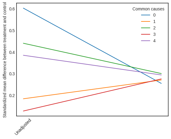
This plot shows how the SMD decreases from the unadjusted to the stratified units.
Method 2: Propensity Score Matching#
We will be using propensity scores to match units in the data.
[11]:
causal_estimate_match = model.estimate_effect(identified_estimand,
                                              method_name="backdoor.propensity_score_matching",
                                              target_units="atc")
print(causal_estimate_match)
print("Causal Estimate is " + str(causal_estimate_match.value))
*** Causal Estimate ***

## Identified estimand
Estimand type: EstimandType.NONPARAMETRIC_ATE

### Estimand : 1
Estimand name: backdoor
Estimand expression:
  d
─────(E[y|W1,W3,W4,W2,W0])
d[v₀]
Estimand assumption 1, Unconfoundedness: If U→{v0} and U→y then P(y|v0,W1,W3,W4,W2,W0,U) = P(y|v0,W1,W3,W4,W2,W0)

## Realized estimand
b: y~v0+W1+W3+W4+W2+W0
Target units: atc

## Estimate
Mean value: 1.0076250251743477

Causal Estimate is 1.0076250251743477
[12]:
# Textual Interpreter
interpretation = causal_estimate_match.interpret(method_name="textual_effect_interpreter")
Increasing the treatment variable(s) [v0] from 0 to 1 causes an increase of 1.0076250251743477 in the expected value of the outcome [['y']], over the data distribution/population represented by the dataset.
Cannot use propensity balance interpretor here since the interpreter method only supports propensity score stratification estimator.
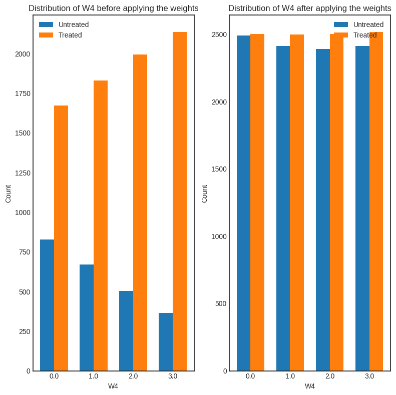
Method 3: Weighting#
We will be using (inverse) propensity scores to assign weights to units in the data. DoWhy supports a few different weighting schemes:
Vanilla Inverse Propensity Score weighting (IPS) (weighting_scheme=”ips_weight”)
Self-normalized IPS weighting (also known as the Hajek estimator) (weighting_scheme=”ips_normalized_weight”)
Stabilized IPS weighting (weighting_scheme = “ips_stabilized_weight”)
[13]:
causal_estimate_ipw = model.estimate_effect(identified_estimand,
                                            method_name="backdoor.propensity_score_weighting",
                                            target_units = "ate",
                                            method_params={"weighting_scheme":"ips_weight"})
print(causal_estimate_ipw)
print("Causal Estimate is " + str(causal_estimate_ipw.value))
*** Causal Estimate ***

## Identified estimand
Estimand type: EstimandType.NONPARAMETRIC_ATE

### Estimand : 1
Estimand name: backdoor
Estimand expression:
  d
─────(E[y|W1,W3,W4,W2,W0])
d[v₀]
Estimand assumption 1, Unconfoundedness: If U→{v0} and U→y then P(y|v0,W1,W3,W4,W2,W0,U) = P(y|v0,W1,W3,W4,W2,W0)

## Realized estimand
b: y~v0+W1+W3+W4+W2+W0
Target units: ate

## Estimate
Mean value: 1.053908836379158

Causal Estimate is 1.053908836379158
[14]:
# Textual Interpreter
interpretation = causal_estimate_ipw.interpret(method_name="textual_effect_interpreter")
Increasing the treatment variable(s) [v0] from 0 to 1 causes an increase of 1.053908836379158 in the expected value of the outcome [['y']], over the data distribution/population represented by the dataset.
[15]:
interpretation = causal_estimate_ipw.interpret(method_name="confounder_distribution_interpreter", fig_size=(8,8), font_size=12, var_name='W4', var_type='discrete')
/home/runner/work/dowhy/dowhy/dowhy/interpreters/confounder_distribution_interpreter.py:83: FutureWarning: The default of observed=False is deprecated and will be changed to True in a future version of pandas. Pass observed=False to retain current behavior or observed=True to adopt the future default and silence this warning.
  barplot_df_before = df.groupby([self.var_name, treated]).size().reset_index(name="count")
/home/runner/work/dowhy/dowhy/dowhy/interpreters/confounder_distribution_interpreter.py:86: FutureWarning: The default of observed=False is deprecated and will be changed to True in a future version of pandas. Pass observed=False to retain current behavior or observed=True to adopt the future default and silence this warning.
  barplot_df_after = df.groupby([self.var_name, treated]).agg({"weight": np.sum}).reset_index()
/home/runner/work/dowhy/dowhy/dowhy/interpreters/confounder_distribution_interpreter.py:86: FutureWarning: The provided callable <function sum at 0x7fea5032e3a0> is currently using SeriesGroupBy.sum. In a future version of pandas, the provided callable will be used directly. To keep current behavior pass the string "sum" instead.
  barplot_df_after = df.groupby([self.var_name, treated]).agg({"weight": np.sum}).reset_index()
[ ]: