Demo for the DoWhy causal API

We show a simple example of adding a causal extension to any dataframe.

import dowhy.datasets
import dowhy.api
from dowhy.graph import build_graph_from_str

import numpy as np
import pandas as pd

from statsmodels.api import OLS

data = dowhy.datasets.linear_dataset(beta=5,
        num_common_causes=1,
        num_instruments = 0,
        num_samples=1000,
        treatment_is_binary=True)
df = data['df']
df['y'] = df['y'] + np.random.normal(size=len(df)) # Adding noise to data. Without noise, the variance in Y|X, Z is zero, and mcmc fails.
nx_graph = build_graph_from_str(data["dot_graph"])

treatment= data["treatment_name"][0]
outcome = data["outcome_name"][0]
common_cause = data["common_causes_names"][0]
df

	W0	v0	y
0	1.734861	True	5.677652
1	1.692967	True	5.345768
2	-0.678012	True	5.865227
3	0.320417	False	-1.465444
4	-1.743889	True	5.025204
...	...	...	...
995	-1.195709	False	-0.097315
996	1.086976	False	1.035984
997	0.115227	True	4.093856
998	0.986937	True	4.631330
999	0.226167	True	5.485148

1000 rows × 3 columns

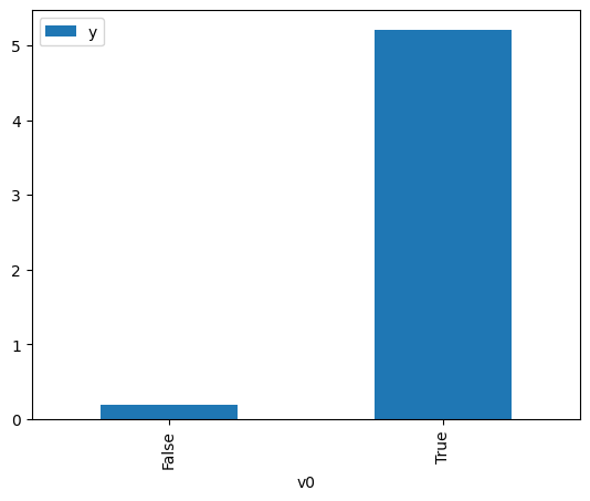
# data['df'] is just a regular pandas.DataFrame
df.causal.do(x=treatment,
             variable_types={treatment: 'b', outcome: 'c', common_cause: 'c'},
             outcome=outcome,
             common_causes=[common_cause],
            ).groupby(treatment).mean().plot(y=outcome, kind='bar')

<Axes: xlabel='v0'>

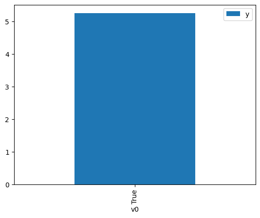
df.causal.do(x={treatment: 1},
              variable_types={treatment:'b', outcome: 'c', common_cause: 'c'},
              outcome=outcome,
              method='weighting',
              common_causes=[common_cause]
              ).groupby(treatment).mean().plot(y=outcome, kind='bar')

<Axes: xlabel='v0'>

cdf_1 = df.causal.do(x={treatment: 1},
              variable_types={treatment: 'b', outcome: 'c', common_cause: 'c'},
              outcome=outcome,
              graph=nx_graph
              )

cdf_0 = df.causal.do(x={treatment: 0},
              variable_types={treatment: 'b', outcome: 'c', common_cause: 'c'},
              outcome=outcome,
              graph=nx_graph
              )

cdf_0

	W0	v0	y	propensity_score	weight
0	1.425122	False	1.553599	0.468980	2.132286
1	1.522968	False	2.940058	0.464910	2.150952
2	1.624560	False	-0.714125	0.460690	2.170659
3	1.883998	False	-1.628021	0.449938	2.222528
4	0.781901	False	-1.317539	0.495812	2.016892
...	...	...	...	...	...
995	1.883998	False	-1.628021	0.449938	2.222528
996	1.624560	False	-0.714125	0.460690	2.170659
997	0.027170	False	1.790618	0.527316	1.896398
998	0.538403	False	-1.014590	0.505985	1.976345
999	0.007696	False	1.750373	0.528127	1.893485

1000 rows × 5 columns

cdf_1

	W0	v0	y	propensity_score	weight
0	1.628855	True	5.879210	0.539489	1.853607
1	0.800083	True	5.501920	0.504947	1.980405
2	1.329587	True	6.044962	0.527042	1.897382
3	2.467841	True	2.798915	0.574072	1.741940
4	0.387281	True	3.828899	0.487704	2.050424
...	...	...	...	...	...
995	2.490357	True	6.209058	0.574992	1.739154
996	0.802514	True	5.794019	0.505049	1.980007
997	0.835262	True	4.489131	0.506417	1.974659
998	0.080196	True	4.995161	0.474894	2.105735
999	1.739403	True	3.959105	0.544075	1.837982

1000 rows × 5 columns

Comparing the estimate to Linear Regression

First, estimating the effect using the causal data frame, and the 95% confidence interval.

(cdf_1['y'] - cdf_0['y']).mean()

$\displaystyle 5.01130335938293$

1.96*(cdf_1['y'] - cdf_0['y']).std() / np.sqrt(len(df))

$\displaystyle 0.0886036474860154$

Comparing to the estimate from OLS.

model = OLS(np.asarray(df[outcome]), np.asarray(df[[common_cause, treatment]], dtype=np.float64))
result = model.fit()
result.summary()

OLS Regression Results

Dep. Variable:	y	R-squared (uncentered):	0.934
Model:	OLS	Adj. R-squared (uncentered):	0.934
Method:	Least Squares	F-statistic:	7086.
Date:	Sat, 12 Jul 2025	Prob (F-statistic):	0.00
Time:	13:59:10	Log-Likelihood:	-1425.1
No. Observations:	1000	AIC:	2854.
Df Residuals:	998	BIC:	2864.
Df Model:	2
Covariance Type:	nonrobust

	coef	std err	t	P>|t|	[0.025	0.975]
x1	0.2809	0.028	9.906	0.000	0.225	0.337
x2	5.0450	0.052	97.125	0.000	4.943	5.147

Omnibus:	1.607	Durbin-Watson:	2.017
Prob(Omnibus):	0.448	Jarque-Bera (JB):	1.600
Skew:	0.047	Prob(JB):	0.449
Kurtosis:	2.828	Cond. No.	2.33

Notes:
[1] R² is computed without centering (uncentered) since the model does not contain a constant.
[2] Standard Errors assume that the covariance matrix of the errors is correctly specified.