Conditional Average Treatment Effects (CATE) with DoWhy and EconML
This is an experimental feature where we use EconML methods from DoWhy. Using EconML allows CATE estimation using different methods.
All four steps of causal inference in DoWhy remain the same: model, identify, estimate, and refute. The key difference is that we now call econml methods in the estimation step. There is also a simpler example using linear regression to understand the intuition behind CATE estimators.
All datasets are generated using linear structural equations.
[1]:
%load_ext autoreload
%autoreload 2
[2]:
import numpy as np
import pandas as pd
import logging

import dowhy
from dowhy import CausalModel
import dowhy.datasets

import econml
import warnings
warnings.filterwarnings('ignore')

BETA = 10
[3]:
data = dowhy.datasets.linear_dataset(BETA, num_common_causes=4, num_samples=10000,
                                    num_instruments=2, num_effect_modifiers=2,
                                     num_treatments=1,
                                    treatment_is_binary=False,
                                    num_discrete_common_causes=2,
                                    num_discrete_effect_modifiers=0,
                                    one_hot_encode=False)
df=data['df']
print(df.head())
print("True causal estimate is", data["ate"])
         X0        X1   Z0        Z1        W0        W1 W2 W3         v0  \
0 -1.264829  1.477951  0.0  0.876127 -1.177224  2.162447  0  0  11.790429
1  0.285403  0.275850  0.0  0.674072 -0.564795  0.205294  2  3  24.917301
2  0.488269  2.793628  0.0  0.293566 -2.104491  2.133887  2  2  18.576141
3  1.128777  0.303312  0.0  0.585147  0.436949  1.515442  2  2  24.540409
4 -0.462207  0.576406  0.0  0.425401 -0.909995 -0.482890  3  1  17.510410

            y
0  188.966111
1  307.304528
2  454.256152
3  322.503760
4  226.807535
True causal estimate is 14.545802196701313
[4]:
model = CausalModel(data=data["df"],
                    treatment=data["treatment_name"], outcome=data["outcome_name"],
                    graph=data["gml_graph"])
[5]:
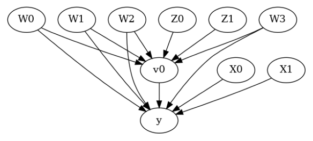
model.view_model()
from IPython.display import Image, display
display(Image(filename="causal_model.png"))
[6]:
identified_estimand= model.identify_effect(proceed_when_unidentifiable=True)
print(identified_estimand)
Estimand type: EstimandType.NONPARAMETRIC_ATE

### Estimand : 1
Estimand name: backdoor
Estimand expression:
  d
─────(E[y|W3,W1,W2,W0])
d[v₀]
Estimand assumption 1, Unconfoundedness: If U→{v0} and U→y then P(y|v0,W3,W1,W2,W0,U) = P(y|v0,W3,W1,W2,W0)

### Estimand : 2
Estimand name: iv
Estimand expression:
 ⎡                              -1⎤
 ⎢    d        ⎛    d          ⎞  ⎥
E⎢─────────(y)⋅⎜─────────([v₀])⎟  ⎥
 ⎣d[Z₀  Z₁]    ⎝d[Z₀  Z₁]      ⎠  ⎦
Estimand assumption 1, As-if-random: If U→→y then ¬(U →→{Z0,Z1})
Estimand assumption 2, Exclusion: If we remove {Z0,Z1}→{v0}, then ¬({Z0,Z1}→y)

### Estimand : 3
Estimand name: frontdoor
No such variable(s) found!
Linear Model
First, let us build some intuition using a linear model for estimating CATE. The effect modifiers (that lead to a heterogeneous treatment effect) can be modeled as interaction terms with the treatment. Thus, their value modulates the effect of treatment.
Below the estimated effect of changing treatment from 0 to 1.
[7]:
linear_estimate = model.estimate_effect(identified_estimand,
                                        method_name="backdoor.linear_regression",
                                       control_value=0,
                                       treatment_value=1)
print(linear_estimate)
*** Causal Estimate ***

## Identified estimand
Estimand type: EstimandType.NONPARAMETRIC_ATE

### Estimand : 1
Estimand name: backdoor
Estimand expression:
  d
─────(E[y|W3,W1,W2,W0])
d[v₀]
Estimand assumption 1, Unconfoundedness: If U→{v0} and U→y then P(y|v0,W3,W1,W2,W0,U) = P(y|v0,W3,W1,W2,W0)

## Realized estimand
b: y~v0+W3+W1+W2+W0+v0*X0+v0*X1
Target units:

## Estimate
Mean value: 14.54571075193559
### Conditional Estimates
__categorical__X0  __categorical__X1
(-3.635, -0.4]     (-3.3569999999999998, 0.0328]     6.738001
                   (0.0328, 0.624]                  10.884184
                   (0.624, 1.129]                   13.391808
                   (1.129, 1.716]                   15.942846
                   (1.716, 4.932]                   20.152733
(-0.4, 0.184]      (-3.3569999999999998, 0.0328]     7.497401
                   (0.0328, 0.624]                  11.566389
                   (0.624, 1.129]                   14.088605
                   (1.129, 1.716]                   16.653022
                   (1.716, 4.932]                   20.751800
(0.184, 0.692]     (-3.3569999999999998, 0.0328]     7.648464
                   (0.0328, 0.624]                  11.935509
                   (0.624, 1.129]                   14.554019
                   (1.129, 1.716]                   17.109583
                   (1.716, 4.932]                   21.116375
(0.692, 1.28]      (-3.3569999999999998, 0.0328]     8.210322
                   (0.0328, 0.624]                  12.459851
                   (0.624, 1.129]                   14.993727
                   (1.129, 1.716]                   17.534435
                   (1.716, 4.932]                   21.836646
(1.28, 4.415]      (-3.3569999999999998, 0.0328]     9.207287
                   (0.0328, 0.624]                  13.083411
                   (0.624, 1.129]                   15.696830
                   (1.129, 1.716]                   18.219924
                   (1.716, 4.932]                   22.366226
dtype: float64
EconML methods
We now move to the more advanced methods from the EconML package for estimating CATE.
First, let us look at the double machine learning estimator. Method_name corresponds to the fully qualified name of the class that we want to use. For double ML, it is “econml.dml.DML”.
Target units defines the units over which the causal estimate is to be computed. This can be a lambda function filter on the original dataframe, a new Pandas dataframe, or a string corresponding to the three main kinds of target units (“ate”, “att” and “atc”). Below we show an example of a lambda function.
Method_params are passed directly to EconML. For details on allowed parameters, refer to the EconML documentation.
[8]:
from sklearn.preprocessing import PolynomialFeatures
from sklearn.linear_model import LassoCV
from sklearn.ensemble import GradientBoostingRegressor
dml_estimate = model.estimate_effect(identified_estimand, method_name="backdoor.econml.dml.DML",
                                     control_value = 0,
                                     treatment_value = 1,
                                 target_units = lambda df: df["X0"]>1,  # condition used for CATE
                                 confidence_intervals=False,
                                method_params={"init_params":{'model_y':GradientBoostingRegressor(),
                                                              'model_t': GradientBoostingRegressor(),
                                                              "model_final":LassoCV(fit_intercept=False),
                                                              'featurizer':PolynomialFeatures(degree=1, include_bias=False)},
                                               "fit_params":{}})
print(dml_estimate)
2023-12-06 08:35:08.848732: I tensorflow/core/platform/cpu_feature_guard.cc:182] This TensorFlow binary is optimized to use available CPU instructions in performance-critical operations.
To enable the following instructions: AVX2 FMA, in other operations, rebuild TensorFlow with the appropriate compiler flags.
2023-12-06 08:35:10.987963: W tensorflow/compiler/tf2tensorrt/utils/py_utils.cc:38] TF-TRT Warning: Could not find TensorRT
*** Causal Estimate ***

## Identified estimand
Estimand type: EstimandType.NONPARAMETRIC_ATE

### Estimand : 1
Estimand name: backdoor
Estimand expression:
  d
─────(E[y|W3,W1,W2,W0])
d[v₀]
Estimand assumption 1, Unconfoundedness: If U→{v0} and U→y then P(y|v0,W3,W1,W2,W0,U) = P(y|v0,W3,W1,W2,W0)

## Realized estimand
b: y~v0+W3+W1+W2+W0 | X0,X1
Target units: Data subset defined by a function

## Estimate
Mean value: 15.637000322550929
Effect estimates: [[12.3018562 ]
 [20.34683672]
 [16.6270295 ]
 ...
 [11.96856018]
 [17.78714676]
 [ 4.99541676]]
[9]:
print("True causal estimate is", data["ate"])
True causal estimate is 14.545802196701313
[10]:
dml_estimate = model.estimate_effect(identified_estimand, method_name="backdoor.econml.dml.DML",
                                     control_value = 0,
                                     treatment_value = 1,
                                 target_units = 1,  # condition used for CATE
                                 confidence_intervals=False,
                                method_params={"init_params":{'model_y':GradientBoostingRegressor(),
                                                              'model_t': GradientBoostingRegressor(),
                                                              "model_final":LassoCV(fit_intercept=False),
                                                              'featurizer':PolynomialFeatures(degree=1, include_bias=True)},
                                               "fit_params":{}})
print(dml_estimate)
*** Causal Estimate ***

## Identified estimand
Estimand type: EstimandType.NONPARAMETRIC_ATE

### Estimand : 1
Estimand name: backdoor
Estimand expression:
  d
─────(E[y|W3,W1,W2,W0])
d[v₀]
Estimand assumption 1, Unconfoundedness: If U→{v0} and U→y then P(y|v0,W3,W1,W2,W0,U) = P(y|v0,W3,W1,W2,W0)

## Realized estimand
b: y~v0+W3+W1+W2+W0 | X0,X1
Target units:

## Estimate
Mean value: 14.475725098861538
Effect estimates: [[15.99699218]
 [11.45432521]
 [23.79690413]
 ...
 [20.39342015]
 [ 5.07113297]
 [20.89578696]]
CATE Object and Confidence Intervals
EconML provides its own methods to compute confidence intervals. Using BootstrapInference in the example below.
[11]:
from sklearn.preprocessing import PolynomialFeatures
from sklearn.linear_model import LassoCV
from sklearn.ensemble import GradientBoostingRegressor
from econml.inference import BootstrapInference
dml_estimate = model.estimate_effect(identified_estimand,
                                     method_name="backdoor.econml.dml.DML",
                                     target_units = "ate",
                                     confidence_intervals=True,
                                     method_params={"init_params":{'model_y':GradientBoostingRegressor(),
                                                              'model_t': GradientBoostingRegressor(),
                                                              "model_final": LassoCV(fit_intercept=False),
                                                              'featurizer':PolynomialFeatures(degree=1, include_bias=True)},
                                               "fit_params":{
                                                               'inference': BootstrapInference(n_bootstrap_samples=100, n_jobs=-1),
                                                            }
                                              })
print(dml_estimate)
*** Causal Estimate ***

## Identified estimand
Estimand type: EstimandType.NONPARAMETRIC_ATE

### Estimand : 1
Estimand name: backdoor
Estimand expression:
  d
─────(E[y|W3,W1,W2,W0])
d[v₀]
Estimand assumption 1, Unconfoundedness: If U→{v0} and U→y then P(y|v0,W3,W1,W2,W0,U) = P(y|v0,W3,W1,W2,W0)

## Realized estimand
b: y~v0+W3+W1+W2+W0 | X0,X1
Target units: ate

## Estimate
Mean value: 14.463127900520695
Effect estimates: [[15.97361844]
 [11.41717088]
 [23.85464337]
 ...
 [20.42508677]
 [ 4.99954998]
 [20.93700213]]
95.0% confidence interval: [[[15.91573366 11.3936291  23.76115269 ... 20.39889196  4.66546959
   20.92996915]]

 [[16.36499412 11.60290173 24.45769177 ... 20.89065299  5.28170646
   21.42348094]]]
Can provide a new inputs as target units and estimate CATE on them.
[12]:
test_cols= data['effect_modifier_names'] # only need effect modifiers' values
test_arr = [np.random.uniform(0,1, 10) for _ in range(len(test_cols))] # all variables are sampled uniformly, sample of 10
test_df = pd.DataFrame(np.array(test_arr).transpose(), columns=test_cols)
dml_estimate = model.estimate_effect(identified_estimand,
                                     method_name="backdoor.econml.dml.DML",
                                     target_units = test_df,
                                     confidence_intervals=False,
                                     method_params={"init_params":{'model_y':GradientBoostingRegressor(),
                                                              'model_t': GradientBoostingRegressor(),
                                                              "model_final":LassoCV(),
                                                              'featurizer':PolynomialFeatures(degree=1, include_bias=True)},
                                               "fit_params":{}
                                              })
print(dml_estimate.cate_estimates)
[[10.61141168]
 [11.44897072]
 [12.8431554 ]
 [13.08904521]
 [11.12794764]
 [10.31407202]
 [14.46399892]
 [13.56944939]
 [15.03914465]
 [11.12365802]]
Can also retrieve the raw EconML estimator object for any further operations
[13]:
print(dml_estimate._estimator_object)
<econml.dml.dml.DML object at 0x7f05e493e970>
Works with any EconML method
In addition to double machine learning, below we example analyses using orthogonal forests, DRLearner (bug to fix), and neural network-based instrumental variables.
Binary treatment, Binary outcome
[14]:
data_binary = dowhy.datasets.linear_dataset(BETA, num_common_causes=4, num_samples=10000,
                                    num_instruments=1, num_effect_modifiers=2,
                                    treatment_is_binary=True, outcome_is_binary=True)
# convert boolean values to {0,1} numeric
data_binary['df'].v0 = data_binary['df'].v0.astype(int)
data_binary['df'].y = data_binary['df'].y.astype(int)
print(data_binary['df'])

model_binary = CausalModel(data=data_binary["df"],
                    treatment=data_binary["treatment_name"], outcome=data_binary["outcome_name"],
                    graph=data_binary["gml_graph"])
identified_estimand_binary = model_binary.identify_effect(proceed_when_unidentifiable=True)
            X0        X1   Z0        W0        W1        W2        W3  v0  y
0    -0.534052  1.093417  0.0 -1.795298 -0.143568 -0.366056 -0.109985   0  0
1    -1.410049  1.026043  0.0  0.492129 -0.119875  3.209130  0.941178   1  1
2    -1.050137 -0.021838  0.0 -0.429270 -0.737206  1.320258  0.804882   1  1
3    -1.587474  0.272291  0.0 -0.816793 -1.156613  0.506778 -0.009565   0  0
4     0.560242  2.063923  0.0  0.404508 -1.074329 -0.733262 -1.824770   0  0
...        ...       ...  ...       ...       ...       ...       ...  .. ..
9995  0.618577  1.331078  1.0 -2.185720  1.263190 -0.412815 -0.395641   0  0
9996 -1.108701  0.171365  1.0  0.974026 -1.133459  1.238863  0.097910   1  1
9997  0.961850  0.630912  0.0  0.881002  0.884787 -0.235011  0.272365   1  1
9998 -1.031732  1.089343  0.0 -0.846813  0.103321  0.483532 -1.245046   0  0
9999 -0.510225  0.689955  0.0 -0.299444  0.434148 -1.397242 -1.944962   0  0

[10000 rows x 9 columns]
Using DRLearner estimator
[15]:
from sklearn.linear_model import LogisticRegressionCV
#todo needs binary y
drlearner_estimate = model_binary.estimate_effect(identified_estimand_binary,
                                method_name="backdoor.econml.dr.LinearDRLearner",
                                confidence_intervals=False,
                                method_params={"init_params":{
                                                    'model_propensity': LogisticRegressionCV(cv=3, solver='lbfgs', multi_class='auto')
                                                    },
                                               "fit_params":{}
                                              })
print(drlearner_estimate)
print("True causal estimate is", data_binary["ate"])
*** Causal Estimate ***

## Identified estimand
Estimand type: EstimandType.NONPARAMETRIC_ATE

### Estimand : 1
Estimand name: backdoor
Estimand expression:
  d
─────(E[y|W3,W1,W2,W0])
d[v₀]
Estimand assumption 1, Unconfoundedness: If U→{v0} and U→y then P(y|v0,W3,W1,W2,W0,U) = P(y|v0,W3,W1,W2,W0)

## Realized estimand
b: y~v0+W3+W1+W2+W0 | X0,X1
Target units: ate

## Estimate
Mean value: 0.3066723343496284
Effect estimates: [[0.35136016]
 [0.21415875]
 [0.2214162 ]
 ...
 [0.55928025]
 [0.27497376]
 [0.33658516]]

True causal estimate is 0.3568
Instrumental Variable Method
[16]:
dmliv_estimate = model.estimate_effect(identified_estimand,
                                        method_name="iv.econml.iv.dml.DMLIV",
                                        target_units = lambda df: df["X0"]>-1,
                                        confidence_intervals=False,
                                method_params={"init_params":{
                                                              'discrete_treatment':False,
                                                              'discrete_instrument':False
                                                             },
                                               "fit_params":{}})
print(dmliv_estimate)
*** Causal Estimate ***

## Identified estimand
Estimand type: EstimandType.NONPARAMETRIC_ATE

### Estimand : 1
Estimand name: iv
Estimand expression:
 ⎡                              -1⎤
 ⎢    d        ⎛    d          ⎞  ⎥
E⎢─────────(y)⋅⎜─────────([v₀])⎟  ⎥
 ⎣d[Z₀  Z₁]    ⎝d[Z₀  Z₁]      ⎠  ⎦
Estimand assumption 1, As-if-random: If U→→y then ¬(U →→{Z0,Z1})
Estimand assumption 2, Exclusion: If we remove {Z0,Z1}→{v0}, then ¬({Z0,Z1}→y)

## Realized estimand
b: y~v0+W3+W1+W2+W0 | X0,X1
Target units: Data subset defined by a function

## Estimate
Mean value: 14.805808316112596
Effect estimates: [[11.69568463]
 [24.05624296]
 [12.39538056]
 ...
 [20.64670216]
 [ 5.13271463]
 [21.08361933]]
Metalearners
[17]:
data_experiment = dowhy.datasets.linear_dataset(BETA, num_common_causes=5, num_samples=10000,
                                    num_instruments=2, num_effect_modifiers=5,
                                    treatment_is_binary=True, outcome_is_binary=False)
# convert boolean values to {0,1} numeric
data_experiment['df'].v0 = data_experiment['df'].v0.astype(int)
print(data_experiment['df'])
model_experiment = CausalModel(data=data_experiment["df"],
                    treatment=data_experiment["treatment_name"], outcome=data_experiment["outcome_name"],
                    graph=data_experiment["gml_graph"])
identified_estimand_experiment = model_experiment.identify_effect(proceed_when_unidentifiable=True)
            X0        X1        X2        X3        X4   Z0        Z1  \
0     1.123930  3.022222 -2.109433  1.328408 -0.840823  1.0  0.129756
1     1.170840 -0.146780 -0.075093  0.175070 -1.536037  0.0  0.040805
2    -0.125031  1.019724  0.711940  1.782758 -1.349459  0.0  0.723018
3     0.558548 -0.440357 -2.302349  0.622907 -0.121145  1.0  0.895617
4     0.531709 -0.699705  1.129274  1.832657 -0.048803  1.0  0.909017
...        ...       ...       ...       ...       ...  ...       ...
9995 -1.189891  0.682024 -0.842743 -1.992564 -1.324105  0.0  0.989291
9996  0.728924 -0.641323 -1.420311  1.217292 -0.844110  1.0  0.318631
9997  0.854360 -0.350899 -0.437845  0.219528 -0.070029  0.0  0.871692
9998 -0.015274  0.875106  0.110283  2.613046  0.361263  0.0  0.374467
9999  1.421508 -0.112686  1.515643  0.511508 -0.292077  1.0  0.958921

            W0        W1        W2        W3        W4  v0          y
0     0.715142 -1.187774 -1.200612 -1.533813  0.776998   1  10.341688
1     1.005776  0.241121 -0.300989  1.710419  2.455758   1  29.654986
2    -2.111568 -0.906330  2.349031 -2.285756  0.161132   1   0.536233
3    -1.424980 -0.751965 -2.018740  0.558397  1.125804   1  -3.399556
4    -1.988515 -2.628349 -0.713607 -0.378804  0.594590   1  -1.203633
...        ...       ...       ...       ...       ...  ..        ...
9995 -1.209167 -1.208427  0.779056  0.994410  2.085716   1   7.089060
9996  0.198992  1.151383  0.363411 -0.938753  2.147780   1  13.943921
9997 -0.587188 -0.903376  0.877840  0.293941  0.779997   1  15.648287
9998 -0.742580 -3.215314 -1.095717 -0.499757 -0.147348   0 -17.576172
9999  0.965338 -0.029347  2.055957 -0.826532 -0.636682   1  24.912374

[10000 rows x 14 columns]
[18]:
from sklearn.ensemble import RandomForestRegressor
metalearner_estimate = model_experiment.estimate_effect(identified_estimand_experiment,
                                method_name="backdoor.econml.metalearners.TLearner",
                                confidence_intervals=False,
                                method_params={"init_params":{
                                                    'models': RandomForestRegressor()
                                                    },
                                               "fit_params":{}
                                              })
print(metalearner_estimate)
print("True causal estimate is", data_experiment["ate"])
*** Causal Estimate ***

## Identified estimand
Estimand type: EstimandType.NONPARAMETRIC_ATE

### Estimand : 1
Estimand name: backdoor
Estimand expression:
  d
─────(E[y|W3,W1,W2,W0,W4])
d[v₀]
Estimand assumption 1, Unconfoundedness: If U→{v0} and U→y then P(y|v0,W3,W1,W2,W0,W4,U) = P(y|v0,W3,W1,W2,W0,W4)

## Realized estimand
b: y~v0+X3+X0+X2+X4+X1+W3+W1+W2+W0+W4
Target units: ate

## Estimate
Mean value: 18.742046322509356
Effect estimates: [[19.90968305]
 [28.05921386]
 [15.12991291]
 ...
 [20.25646756]
 [17.54863467]
 [26.25831746]]

True causal estimate is 11.548902280318803
Avoiding retraining the estimator
Once an estimator is fitted, it can be reused to estimate effect on different data points. In this case, you can pass fit_estimator=False to estimate_effect. This works for any EconML estimator. We show an example for the T-learner below.
[19]:
# For metalearners, need to provide all the features (except treatmeant and outcome)
metalearner_estimate = model_experiment.estimate_effect(identified_estimand_experiment,
                                method_name="backdoor.econml.metalearners.TLearner",
                                confidence_intervals=False,
                                fit_estimator=False,
                                target_units=data_experiment["df"].drop(["v0","y", "Z0", "Z1"], axis=1)[9995:],
                                method_params={})
print(metalearner_estimate)
print("True causal estimate is", data_experiment["ate"])
*** Causal Estimate ***

## Identified estimand
Estimand type: EstimandType.NONPARAMETRIC_ATE

### Estimand : 1
Estimand name: backdoor
Estimand expression:
  d
─────(E[y|W3,W1,W2,W0,W4])
d[v₀]
Estimand assumption 1, Unconfoundedness: If U→{v0} and U→y then P(y|v0,W3,W1,W2,W0,W4,U) = P(y|v0,W3,W1,W2,W0,W4)

## Realized estimand
b: y~v0+X3+X0+X2+X4+X1+W3+W1+W2+W0+W4
Target units: Data subset provided as a data frame

## Estimate
Mean value: 18.71229118037352
Effect estimates: [[14.69208446]
 [14.80595175]
 [20.25646756]
 [17.54863467]
 [26.25831746]]

True causal estimate is 11.548902280318803
Refuting the estimate
Adding a random common cause variable
[20]:
res_random=model.refute_estimate(identified_estimand, dml_estimate, method_name="random_common_cause")
print(res_random)
Refute: Add a random common cause
Estimated effect:12.363085365933857
New effect:12.341220390740773
p value:0.46
Adding an unobserved common cause variable
[21]:
res_unobserved=model.refute_estimate(identified_estimand, dml_estimate, method_name="add_unobserved_common_cause",
                                     confounders_effect_on_treatment="linear", confounders_effect_on_outcome="linear",
                                    effect_strength_on_treatment=0.01, effect_strength_on_outcome=0.02)
print(res_unobserved)
Refute: Add an Unobserved Common Cause
Estimated effect:12.363085365933857
New effect:12.325334320191756
Replacing treatment with a random (placebo) variable
[22]:
res_placebo=model.refute_estimate(identified_estimand, dml_estimate,
        method_name="placebo_treatment_refuter", placebo_type="permute",
        num_simulations=10 # at least 100 is good, setting to 10 for speed
        )
print(res_placebo)
Refute: Use a Placebo Treatment
Estimated effect:12.363085365933857
New effect:0.012137033388297663
p value:0.31953547192756526
Removing a random subset of the data
[23]:
res_subset=model.refute_estimate(identified_estimand, dml_estimate,
        method_name="data_subset_refuter", subset_fraction=0.8,
        num_simulations=10)
print(res_subset)
Refute: Use a subset of data
Estimated effect:12.363085365933857
New effect:12.315879364150556
p value:0.03437419719145829
More refutation methods to come, especially specific to the CATE estimators.