Attributing Distributional Changes

When attributing distribution changes, we answer the question:

What mechanism in my system changed between two sets of data? Or in other words, which node in my data behaves differently?

Here we want to identify the node or nodes in the graph where the causal mechanism has changed. For example, if we detect an uptick in latency of our application within a microservice architecture, we aim to identify the node/component whose behavior has altered. has changed. DoWhy implements a method to identify and attribute changes in a distribution to changes in causal mechanisms of upstream nodes following the paper:

Kailash Budhathoki, Dominik Janzing, Patrick Blöbaum, Hoiyi Ng. Why did the distribution change? Proceedings of The 24th International Conference on Artificial Intelligence and Statistics, PMLR 130:1666-1674, 2021.

How to use it

To see how to use the method, let’s take the microservice example from above and assume we have a system of four services $X, Y, Z, W$ , each of which monitors latencies. Suppose we plan to carry out a new deployment and record the latencies before and after the deployment. We will refer to the latency data gathered prior to the deployment as data_old and the data gathered after the deployment as data_new:

>>> import networkx as nx, numpy as np, pandas as pd
>>> from dowhy import gcm
>>> from scipy.stats import halfnorm

>>> X = halfnorm.rvs(size=1000, loc=0.5, scale=0.2)
>>> Y = halfnorm.rvs(size=1000, loc=1.0, scale=0.2)
>>> Z = np.maximum(X, Y) + np.random.normal(loc=0, scale=0.5, size=1000)
>>> W = Z + halfnorm.rvs(size=1000, loc=0.1, scale=0.2)
>>> data_old = pd.DataFrame(data=dict(X=X, Y=Y, Z=Z, W=W))

>>> X = halfnorm.rvs(size=1000, loc=0.5, scale=0.2)
>>> Y = halfnorm.rvs(size=1000, loc=1.0, scale=0.2)
>>> Z = X + Y + np.random.normal(loc=0, scale=0.5, size=1000)
>>> W = Z + halfnorm.rvs(size=1000, loc=0.1, scale=0.2)
>>> data_new = pd.DataFrame(data=dict(X=X, Y=Y, Z=Z, W=W))

Here, we change the behaviour of $Z$ , which simulates an accidental conversion of multi-threaded code into sequential one (waiting for $X$ and $Y$ in parallel vs. waiting for them sequentially). This will change the distribution of $Z$ and subsequently $W$ .

Next, we’ll model cause-effect relationships as a probabilistic causal model:

>>> causal_model = gcm.ProbabilisticCausalModel(nx.DiGraph([('X', 'Z'), ('Y', 'Z'), ('Z', 'W')]))  # (X, Y) -> Z -> W
>>> gcm.auto.assign_causal_mechanisms(causal_model, data_old)

Finally, we attribute changes in distributions of $W$ to changes in causal mechanisms:

>>> attributions = gcm.distribution_change(causal_model, data_old, data_new, 'W')
>>> attributions
{'W': 0.012553173521649849, 'X': -0.007493424287710609, 'Y': 0.0013256550695736396, 'Z': 0.7396701922473544}

Although the distribution of $W$ has changed as well, the method attributes the change almost completely to $Z$ with negligible scores for the other variables. This is in line with our expectations since we only altered the mechanism of $Z$ . Note that the unit of the scores depends on the used measure (see the next section).

As the reader may have noticed, there is no fitting step involved when using this method. The reason is, that this function will call fit internally. To be precise, this function will make two copies of the causal graph and fit one graph to the first dataset and the second graph to the second dataset.

Understanding the method

The idea behind this method is to systematically replace the causal mechanism learned based on the old dataset with the mechanism learned based on the new dataset. After each replacement, new samples are generated for the target node, where the data generation process is a mixture of old and new mechanisms. Our goal is to identify the mechanisms that have changed, which would lead to a different marginal distribution of the target, while unchanged mechanisms would result in the same marginal distribution. To achieve this, we employ the idea of a Shapley symmetrization to systematically replace the mechanisms. This enables us to identify which nodes have changed and to estimate an attribution score with respect to some measure. Note that a change in the mechanism could be due to a functional change in the underlying model or a change in the (unobserved) noise distribution. However, both changes would lead to a change in the mechanism.

The steps here are as follows:

Estimate the conditional distributions from ‘old’ data (e.g., latencies before deployment): $P_{X_{1}, . . ., X_{n}} = \prod_{j} P_{X_{j} | P A_{j}}$ , where $P_{X_{j} | P A_{j}}$ is the causal mechanism of node $X_{j}$ and $P A_{j}$ the parents of node $X_{j}$
Estimate the conditional distributions from ‘new’ data (e.g., latencies after deployment): ${\tilde{P}}_{X_{1}, . . ., X_{n}} = \prod_{j} {\tilde{P}}_{X_{j} | P A_{j}}$
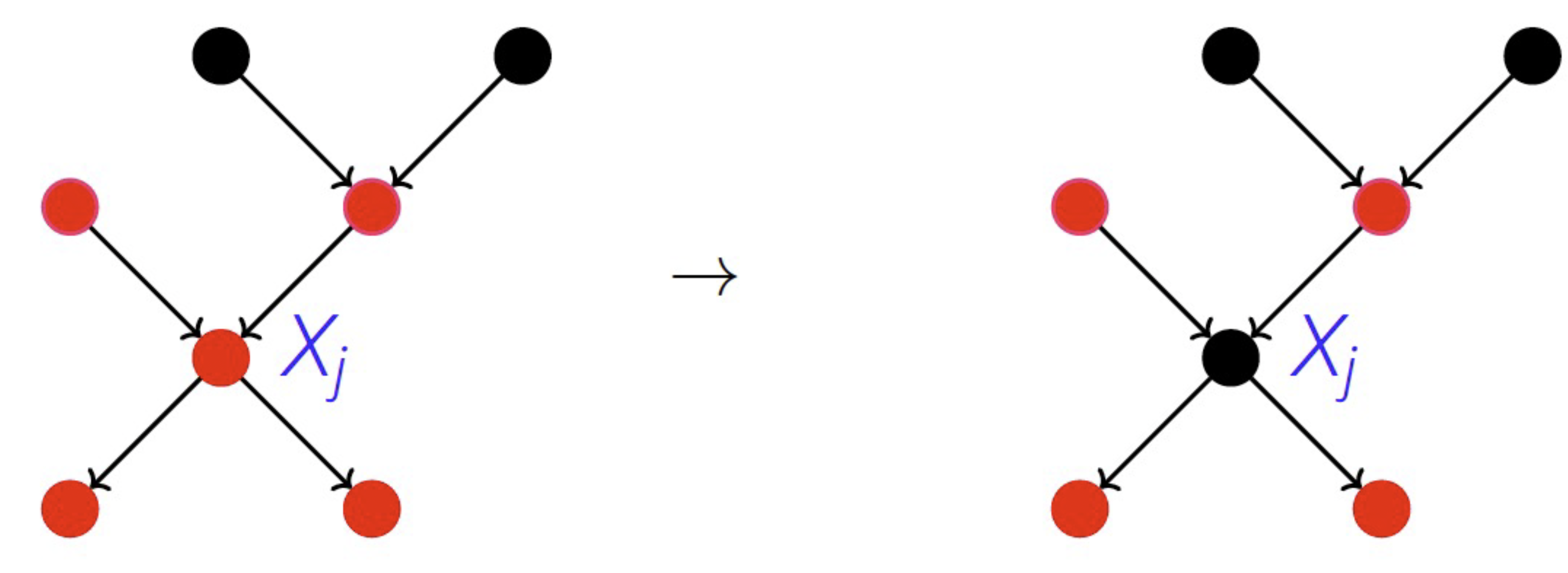
Replace mechanisms based on the ‘old’ data with mechanisms based on the ‘new’ data systematically, one by one. For this, replace $P_{X_{j} | P A_{j}}$ by ${\tilde{P}}_{X_{j} | P A_{j}}$ for each $j$ . If nodes in $T \subseteq {1, . . ., n}$ have been replaced before, we get ${\tilde{P}}_{T}^{X_{n}} = \sum_{x_{1}, . . ., x_{n - 1}} \prod_{j \in T} {\tilde{P}}_{X_{j} | P A_{j}} \prod_{j \notin T} P_{X_{j} | P A_{j}}$ , a new marginal for node $n$ .
Attribute the change in the marginal given $T$ to $X_{j}$ using Shapley values by comparing $P_{T ⋃ {j}}^{X_{n}}$ and $P_{T}^{X_{n}}$ . Here, we can use different measures to capture the change, such as KL divergence to the original distribution or difference in variances etc.

For more detailed explanation, see the corresponding paper: Why did the distribution change?