Estimating effect of multiple treatments
[1]:
from dowhy import CausalModel
import dowhy.datasets

import warnings
warnings.filterwarnings('ignore')
[2]:
data = dowhy.datasets.linear_dataset(10, num_common_causes=4, num_samples=10000,
                                     num_instruments=0, num_effect_modifiers=2,
                                     num_treatments=2,
                                     treatment_is_binary=False,
                                     num_discrete_common_causes=2,
                                     num_discrete_effect_modifiers=0,
                                     one_hot_encode=False)
df=data['df']
df.head()
[2]:
| X0 | X1 | W0 | W1 | W2 | W3 | v0 | v1 | y | |
|---|---|---|---|---|---|---|---|---|---|
| 0 | -2.021017 | -0.720521 | -0.679301 | -1.139210 | 2 | 0 | 3.444861 | 4.527003 | -81.852189 |
| 1 | -1.559724 | -0.896530 | 0.796469 | 0.290310 | 2 | 3 | 14.298551 | 18.611908 | -2060.112833 |
| 2 | -1.813168 | -3.164663 | -2.179785 | 0.963711 | 1 | 1 | -4.688412 | 7.647699 | 568.243251 |
| 3 | -2.311118 | -0.838924 | -1.082225 | 1.124652 | 2 | 1 | 5.035879 | 12.740790 | -606.968110 |
| 4 | -0.806821 | 1.177355 | 0.085482 | 0.545155 | 2 | 0 | 9.000252 | 9.347315 | 85.136811 |
[3]:
model = CausalModel(data=data["df"],
                    treatment=data["treatment_name"], outcome=data["outcome_name"],
                    graph=data["gml_graph"])
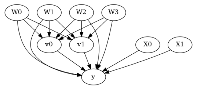
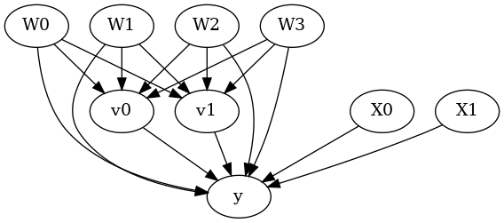
[4]:
model.view_model()
from IPython.display import Image, display
display(Image(filename="causal_model.png"))
[5]:
identified_estimand= model.identify_effect(proceed_when_unidentifiable=True)
print(identified_estimand)
Estimand type: EstimandType.NONPARAMETRIC_ATE

### Estimand : 1
Estimand name: backdoor
Estimand expression:
    d
─────────(E[y|W3,W2,W0,W1])
d[v₀  v₁]
Estimand assumption 1, Unconfoundedness: If U→{v0,v1} and U→y then P(y|v0,v1,W3,W2,W0,W1,U) = P(y|v0,v1,W3,W2,W0,W1)

### Estimand : 2
Estimand name: iv
No such variable(s) found!

### Estimand : 3
Estimand name: frontdoor
No such variable(s) found!
Linear model
Let us first see an example for a linear model. The control_value and treatment_value can be provided as a tuple/list when the treatment is multi-dimensional.
The interpretation is change in y when v0 and v1 are changed from (0,0) to (1,1).
[6]:
linear_estimate = model.estimate_effect(identified_estimand,
                                        method_name="backdoor.linear_regression",
                                        control_value=(0,0),
                                        treatment_value=(1,1),
                                        method_params={'need_conditional_estimates': False})
print(linear_estimate)
*** Causal Estimate ***

## Identified estimand
Estimand type: EstimandType.NONPARAMETRIC_ATE

### Estimand : 1
Estimand name: backdoor
Estimand expression:
    d
─────────(E[y|W3,W2,W0,W1])
d[v₀  v₁]
Estimand assumption 1, Unconfoundedness: If U→{v0,v1} and U→y then P(y|v0,v1,W3,W2,W0,W1,U) = P(y|v0,v1,W3,W2,W0,W1)

## Realized estimand
b: y~v0+v1+W3+W2+W0+W1+v0*X1+v0*X0+v1*X1+v1*X0
Target units: ate

## Estimate
Mean value: -99.2119565887595
You can estimate conditional effects, based on effect modifiers.
[7]:
linear_estimate = model.estimate_effect(identified_estimand,
                                        method_name="backdoor.linear_regression",
                                        control_value=(0,0),
                                        treatment_value=(1,1))
print(linear_estimate)
*** Causal Estimate ***

## Identified estimand
Estimand type: EstimandType.NONPARAMETRIC_ATE

### Estimand : 1
Estimand name: backdoor
Estimand expression:
    d
─────────(E[y|W3,W2,W0,W1])
d[v₀  v₁]
Estimand assumption 1, Unconfoundedness: If U→{v0,v1} and U→y then P(y|v0,v1,W3,W2,W0,W1,U) = P(y|v0,v1,W3,W2,W0,W1)

## Realized estimand
b: y~v0+v1+W3+W2+W0+W1+v0*X1+v0*X0+v1*X1+v1*X0
Target units:

## Estimate
Mean value: -99.2119565887595
### Conditional Estimates
__categorical__X1  __categorical__X0
(-4.351, -1.605]   (-5.191000000000001, -1.865]   -247.195514
                   (-1.865, -1.253]               -183.266013
                   (-1.253, -0.745]               -144.589016
                   (-0.745, -0.133]               -105.180955
                   (-0.133, 2.526]                 -36.829845
(-1.605, -1.014]   (-5.191000000000001, -1.865]   -218.135497
                   (-1.865, -1.253]               -154.088112
                   (-1.253, -0.745]               -115.554759
                   (-0.745, -0.133]                -77.113437
                   (-0.133, 2.526]                 -15.252452
(-1.014, -0.525]   (-5.191000000000001, -1.865]   -203.497190
                   (-1.865, -1.253]               -137.140692
                   (-1.253, -0.745]                -98.253212
                   (-0.745, -0.133]                -59.661888
                   (-0.133, 2.526]                   3.601806
(-0.525, 0.0526]   (-5.191000000000001, -1.865]   -185.622389
                   (-1.865, -1.253]               -121.280612
                   (-1.253, -0.745]                -81.134375
                   (-0.745, -0.133]                -42.248661
                   (-0.133, 2.526]                  18.743879
(0.0526, 3.03]     (-5.191000000000001, -1.865]   -158.649349
                   (-1.865, -1.253]                -92.683045
                   (-1.253, -0.745]                -56.037456
                   (-0.745, -0.133]                -15.141187
                   (-0.133, 2.526]                  46.139026
dtype: float64
More methods
You can also use methods from EconML or CausalML libraries that support multiple treatments. You can look at examples from the conditional effect notebook: https://py-why.github.io/dowhy/example_notebooks/dowhy-conditional-treatment-effects.html
Propensity-based methods do not support multiple treatments currently.